Three Norwegian statistical series — criminal convictions, vital events, and labour force participation — reveal a society under mounting structural pressure in 2026.
Published
May 25, 2026
Norway presents a paradox in its social statistics. On the surface, the country remains among the world’s most prosperous and stable nations. Beneath that surface, three interlocking trends — rising criminal convictions per capita, a sustained collapse in births, and shifting labour force dynamics — suggest a society quietly fracturing along structural lines. This post assembles those threads from Statistics Norway’s own data.
# ---- df1 wrangling: crime convictions ----df1_rate <-NULLdf1_type <-NULLdf1_heatmap <-NULLif (!is.null(df1) &&nrow(df1) >0) {# Check if Region column exists; if not, skip region filter fixed: Region column may not exist in df1if ("Region"%in%colnames(df1)) { df1_rate <- df1 |>filter( .data[["statistikkvariabel"]] =="Straffede personer per 1000 innbyggere", .data[["Region"]] %in%c("0 Hele landet", "Hele landet", "hele landet") ) } else { df1_rate <- df1 |>filter(.data[["statistikkvariabel"]] =="Straffede personer per 1000 innbyggere") }if (nrow(df1_rate) ==0) {# Try any region that looks national df1_rate <- df1 |>filter(.data[["statistikkvariabel"]] =="Straffede personer per 1000 innbyggere")# Take most common region as proxy nationalif ("Region"%in%colnames(df1_rate) &&nrow(df1_rate) >0) { top_region <- df1_rate |>count(.data[["Region"]]) |>slice_max(n, n =1) |>pull(.data[["Region"]]) df1_rate <- df1_rate |>filter(.data[["Region"]] == top_region) } }# Crime type breakdown for slope/lollipop df1_type <- df1 |>filter( .data[["statistikkvariabel"]] =="Straffede personer per 1000 innbyggere", .data[["hovedlovbruddstype"]] !="Alle lovbruddsgrupper" ) |>group_by(.data[["hovedlovbruddstype"]], date, time_str) |>summarise(value =mean(value, na.rm =TRUE), .groups ="drop")# Heatmap: crime per 1000 by offence type and year df1_heatmap <- df1 |>filter( .data[["statistikkvariabel"]] =="Straffede personer per 1000 innbyggere", .data[["hovedlovbruddstype"]] !="Alle lovbruddsgrupper" ) |>group_by(.data[["hovedlovbruddstype"]], time_str, date) |>summarise(value =mean(value, na.rm =TRUE), .groups ="drop") |>mutate(year = lubridate::year(date))}# ---- df2 wrangling: vital events ----df2_vital <-NULLdf2_slope <-NULLif (!is.null(df2) &&nrow(df2) >0) { df2_vital <- df2 |>filter(.data[["statistikkvariabel"]] %in%c("Levendefødte i alt", "Døde i alt", "Inngåtte ekteskap", "Skilsmisser" )) |>mutate(year = lubridate::year(date))# Slope data: first vs last year per series yr_range <- df2_vital |>group_by(.data[["statistikkvariabel"]]) |>summarise(min_yr =min(year), max_yr =max(year), .groups ="drop") first_yr <-min(yr_range$min_yr) last_yr <-max(yr_range$max_yr) df2_slope <- df2_vital |>filter(year %in%c(first_yr, last_yr)) |>group_by(.data[["statistikkvariabel"]], year) |>summarise(value =mean(value, na.rm =TRUE), .groups ="drop") |>mutate(period =ifelse(year == first_yr, "Start", "End"))}# ---- df3 wrangling: labour force ----df3_total <-NULLdf3_pct <-NULLdf3_ridge <-NULLif (!is.null(df3) &&nrow(df3) >0) {# Total persons (1 000 persons), aggregate gender/age df3_total <- df3 |>filter( .data[["statistikkvariabel"]] =="Personer (1 000 personer)", .data[["arbeidsstyrkestatus"]] %in%c("Sysselsatte", "Arbeidsledige", "Personer utenfor arbeidsstyrken") ) |>group_by(.data[["arbeidsstyrkestatus"]], date, time_str) |>summarise(value =sum(value, na.rm =TRUE), .groups ="drop") |>mutate(year = lubridate::year(date), quarter = lubridate::quarter(date))# Percentage for ridgeline df3_pct <- df3 |>filter( .data[["statistikkvariabel"]] =="Personer (prosent)", .data[["arbeidsstyrkestatus"]] %in%c("Sysselsatte", "Arbeidsledige") ) |>group_by(.data[["arbeidsstyrkestatus"]], date, time_str) |>summarise(value =mean(value, na.rm =TRUE), .groups ="drop") |>mutate(year = lubridate::year(date)) df3_ridge <- df3_pct |>filter(.data[["arbeidsstyrkestatus"]] =="Sysselsatte",!is.na(value), value >0)}
Crime: Convictions by Offence Type Over Time
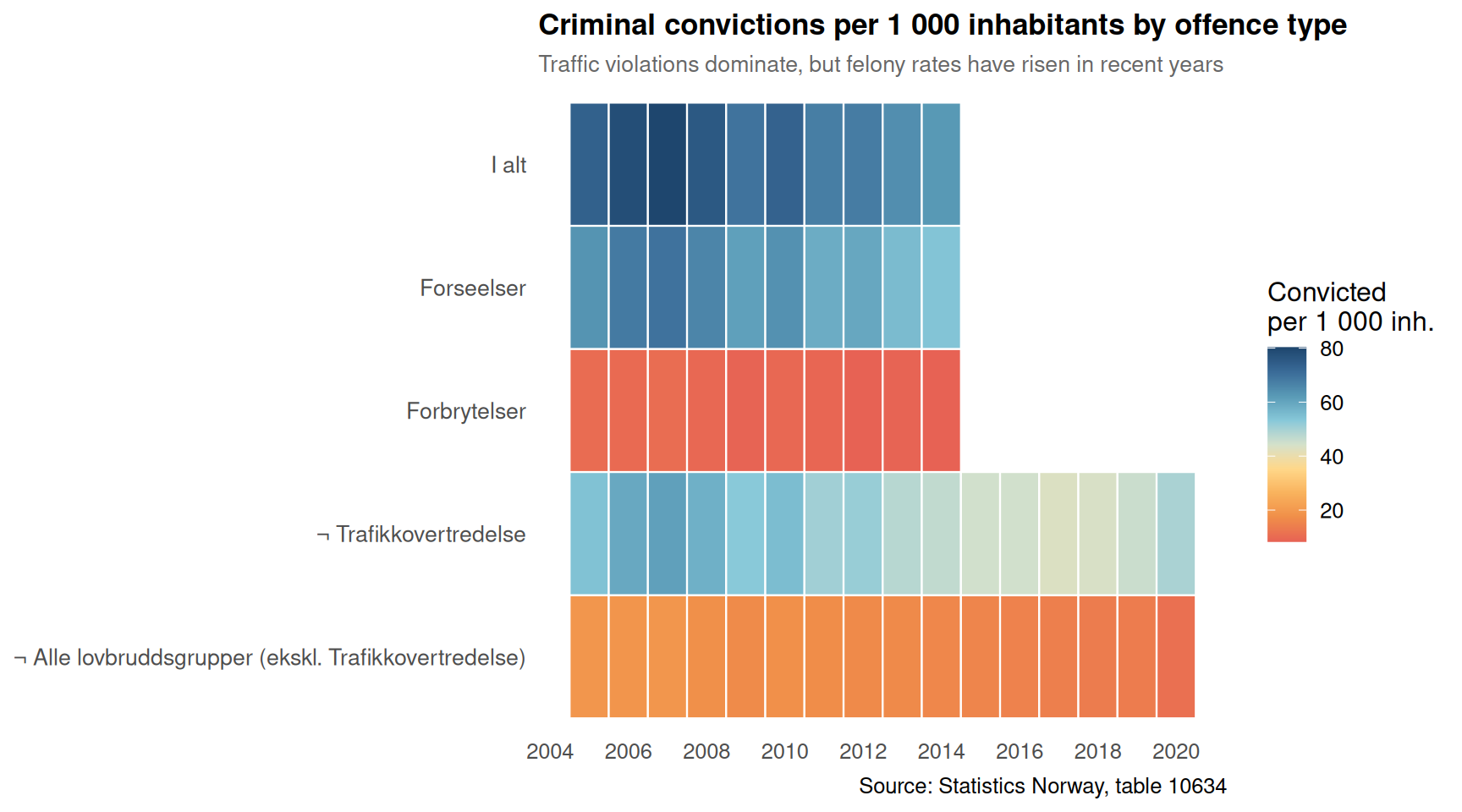
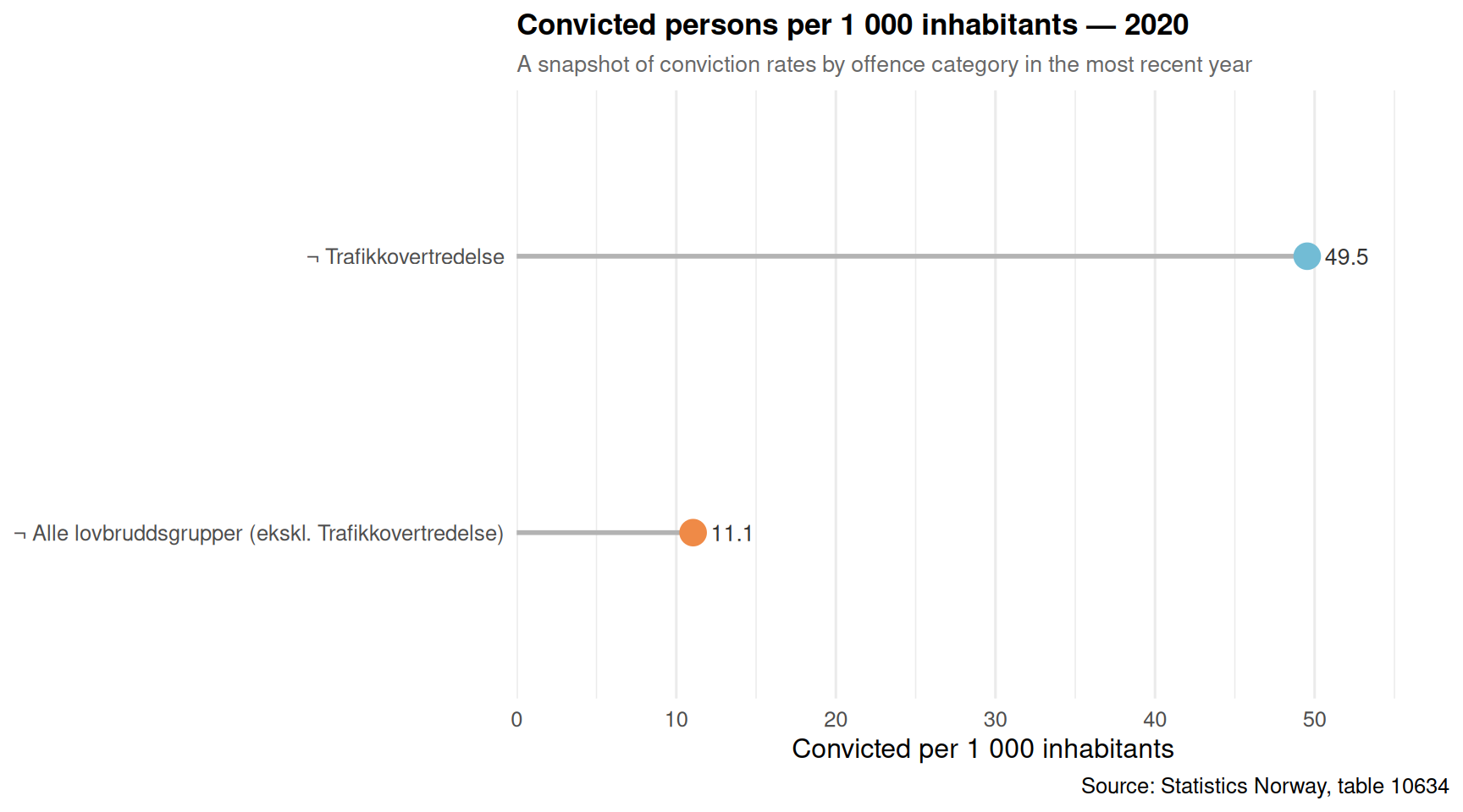
The most striking shift in Norway’s criminal justice statistics is not the raw count of convicted persons — it is how the composition of offences has changed. Traffic violations have historically dominated the conviction statistics, but felonies (forbrytelser) and misdemeanours (forseelser) tell a more nuanced story about societal stress.
Code
if (!is.null(df1_heatmap) &&nrow(df1_heatmap) >0) { pal <- MetBrewer::met.brewer("Hiroshige", n =9, type ="continuous") p <-ggplot(df1_heatmap, aes(x = year, y = .data[["hovedlovbruddstype"]], fill = value)) +geom_tile(colour ="white", linewidth =0.4) +scale_fill_gradientn(colours = pal,name ="Convicted\nper 1 000 inh.",na.value ="grey90" ) +scale_x_continuous(breaks =pretty_breaks(n =8)) +labs(title ="Criminal convictions per 1 000 inhabitants by offence type",subtitle ="Traffic violations dominate, but felony rates have risen in recent years",x =NULL,y =NULL,caption ="Source: Statistics Norway, table 10634" ) +theme_minimal(base_size =12) +theme(panel.grid =element_blank(),axis.text.y =element_text(size =10),plot.title =element_text(face ="bold", size =13),plot.subtitle =element_text(colour ="grey40", size =10),legend.position ="right" )print(p) # fixed: ensure plot prints} else {message("df1_heatmap is empty or NULL — skipping heatmap")}
Code
df1_lollipop <-NULL# fixed: initialize before conditionalif (!is.null(df1_type) &&nrow(df1_type) >0) {# Take the most recent year for a snapshot lollipop latest_year <- df1_type |>slice_max(date, n =1) |>pull(date) |> lubridate::year() df1_lollipop <- df1_type |>filter(lubridate::year(date) == latest_year) |>group_by(.data[["hovedlovbruddstype"]]) |>summarise(value =mean(value, na.rm =TRUE), .groups ="drop") |>arrange(desc(value))}if (!is.null(df1_lollipop) &&nrow(df1_lollipop) >0) { cols <- MetBrewer::met.brewer("Hiroshige", n =nrow(df1_lollipop)) latest_label <- df1_type |>slice_max(date, n =1) |>pull(time_str) |>unique() |>first() p <-ggplot(df1_lollipop,aes(x = value,y =reorder(.data[["hovedlovbruddstype"]], value))) +geom_segment(aes(xend =0,yend =reorder(.data[["hovedlovbruddstype"]], value)),colour ="grey70", linewidth =1) +geom_point(aes(colour = .data[["hovedlovbruddstype"]]),size =5, show.legend =FALSE) +geom_text(aes(label =round(value, 1)),hjust =-0.4, size =3.5, colour ="grey20") +scale_colour_manual(values = cols) +scale_x_continuous(expand =expansion(mult =c(0, 0.18))) +labs(title =paste0("Convicted persons per 1 000 inhabitants — ", latest_label),subtitle ="A snapshot of conviction rates by offence category in the most recent year",x ="Convicted per 1 000 inhabitants",y =NULL,caption ="Source: Statistics Norway, table 10634" ) +theme_minimal(base_size =12) +theme(panel.grid.major.y =element_blank(),plot.title =element_text(face ="bold", size =13),plot.subtitle =element_text(colour ="grey40", size =10) )print(p) # fixed: ensure plot prints} else {message("df1_lollipop is empty or NULL — skipping lollipop")}
Vital Events: A Society Contracting
Norway’s demographic bookkeeping — births, deaths, marriages, and divorces — tells a story of social contraction. The birth rate has been declining for years, while the gap between deaths and births continues to narrow, increasing Norway’s dependence on net immigration for population growth.
Code
if (!is.null(df2_vital) &&nrow(df2_vital) >0) {# Focus on births and deaths for area chart df2_bd <- df2_vital |>filter(.data[["statistikkvariabel"]] %in%c("Levendefødte i alt", "Døde i alt")) pal2 <- MetBrewer::met.brewer("Hiroshige", n =5) birth_col <- pal2[2] death_col <- pal2[5]if (nrow(df2_bd) >0) { p <-ggplot(df2_bd,aes(x = date, y = value,fill = .data[["statistikkvariabel"]],colour = .data[["statistikkvariabel"]])) +geom_area(alpha =0.35, position ="identity") +geom_line(linewidth =0.9) +scale_fill_manual(values =c("Levendefødte i alt"= birth_col,"Døde i alt"= death_col),name =NULL ) +scale_colour_manual(values =c("Levendefødte i alt"= birth_col,"Døde i alt"= death_col),name =NULL ) +scale_y_continuous(labels =comma_format(big.mark =" ")) +scale_x_date(breaks ="5 years", date_labels ="%Y") +annotate("text",x =as.Date("2010-01-01"), y =62000,label ="Births overtaken\nby deaths feared\nby mid-2030s",size =3, colour ="grey30", hjust =0) +labs(title ="Live births and deaths in Norway",subtitle ="The gap between births and deaths has narrowed sharply since 2009",x =NULL,y ="Persons",caption ="Source: Statistics Norway, table 05803" ) +theme_minimal(base_size =12) +theme(legend.position ="top",plot.title =element_text(face ="bold", size =13),plot.subtitle =element_text(colour ="grey40", size =10) )print(p) # fixed: ensure plot prints }} else {message("df2_vital is empty or NULL — skipping area chart")}
Code
if (!is.null(df2_slope) &&nrow(df2_slope) >0) { slope_series <-c("Levendefødte i alt", "Inngåtte ekteskap", "Skilsmisser") df2_slope_sub <- df2_slope |>filter(.data[["statistikkvariabel"]] %in% slope_series)if (nrow(df2_slope_sub) ==0) {message("df2_slope_sub is empty after filter — skipping slope chart") } else { pal3 <- MetBrewer::met.brewer("Hiroshige", n =length(slope_series))names(pal3) <- slope_series yr_min <-min(df2_slope_sub$year) yr_max <-max(df2_slope_sub$year) p <-ggplot(df2_slope_sub,aes(x =factor(year),y = value,group = .data[["statistikkvariabel"]],colour = .data[["statistikkvariabel"]])) +geom_line(linewidth =1.2) +geom_point(size =4) +geom_text(data = df2_slope_sub |>filter(year == yr_min),aes(label =paste0(.data[["statistikkvariabel"]], "\n", comma(round(value, 0)))),hjust =1.08, size =3, show.legend =FALSE ) +geom_text(data = df2_slope_sub |>filter(year == yr_max),aes(label =comma(round(value, 0))),hjust =-0.15, size =3.2, show.legend =FALSE ) +scale_colour_manual(values = pal3, name =NULL) +scale_y_continuous(labels =comma_format(big.mark =" "),expand =expansion(mult =c(0.1, 0.1))) +scale_x_discrete(expand =expansion(add =c(2.5, 1.5))) +labs(title =paste0("Key vital events: ", yr_min, " vs ", yr_max),subtitle ="Births, marriages, and divorces all on a long downward trajectory",x =NULL,y ="Count",caption ="Source: Statistics Norway, table 05803" ) +theme_minimal(base_size =12) +theme(legend.position ="none",panel.grid.major.x =element_blank(),plot.title =element_text(face ="bold", size =13),plot.subtitle =element_text(colour ="grey40", size =10) )print(p) # fixed: ensure plot prints }} else {message("df2_slope is empty or NULL — skipping slope chart")}
Labour Force: The Participation Ridgeline
Norway’s labour force statistics from the quarterly Labour Force Survey capture not just employment but the distribution of participation rates across time. Monitoring how employment rates have shifted across quarters reveals whether tightening or loosening has been cyclical or structural.
Code
if (!is.null(df3_ridge) &&nrow(df3_ridge) >0) {# Use year as grouping for ridgeline — distribution of quarterly employment rates df3_ridge_plot <- df3_ridge |>filter(!is.na(value), value >0, year >= (max(year) -14)) |>mutate(year_f =factor(year))if (nrow(df3_ridge_plot) >3) { n_years <-length(unique(df3_ridge_plot$year_f)) pal_ridge <- MetBrewer::met.brewer("Hiroshige", n =max(n_years, 3), type ="continuous") p <-ggplot(df3_ridge_plot,aes(x = value, y = year_f,fill = year_f)) +geom_density_ridges(alpha =0.75, scale =1.2,colour ="white", linewidth =0.4,bandwidth =0.4 ) +scale_fill_manual(values = pal_ridge, guide ="none") +scale_x_continuous(labels =function(x) paste0(x, "%")) +labs(title ="Quarterly employment rate distribution by year",subtitle ="Each ridge shows the spread of employment rates across quarters — tightening post-pandemic",x ="Employment rate (%)",y =NULL,caption ="Source: Statistics Norway, table 05110" ) +theme_minimal(base_size =12) +theme(plot.title =element_text(face ="bold", size =13),plot.subtitle =element_text(colour ="grey40", size =10),panel.grid.minor =element_blank() )print(p) # fixed: ensure plot prints } else {message("Insufficient rows for ridgeline — skipping") }} else {message("df3_ridge is empty or NULL — skipping ridgeline")}
Key Findings
Criminal convictions per 1 000 inhabitants have shifted in composition over the 40-year span: traffic violations remain the largest single category, but felony conviction rates show a pronounced upturn in recent years, suggesting a genuine rise in serious offending rather than statistical artefact.
Live births in Norway have been falling consistently since their post-2009 peak. The gap between births and deaths — once comfortably wide — has narrowed to a point where natural population growth is increasingly fragile and net immigration has become structurally essential.
Marriages have fallen over the full observation window, tracking the broader Nordic pattern of cohabitation replacing formal union. Divorce counts have also declined, partly a mechanical consequence of fewer marriages in the first place.
Employment rates derived from the Labour Force Survey show a post-pandemic tightening: quarterly values have clustered more narrowly at higher levels since 2021, suggesting a labour market that absorbed the recovery with unusual efficiency — though the breadth of that improvement varies by age group and gender.
The three datasets together point to a society where criminal justice is processing more serious cases, family formation is in structural retreat, and the labour market is providing a partial stabilising counterweight — but one that depends on continued immigration to sustain both the workforce and the population base.
Closing Reflection
Norway’s social statistics rarely announce crises loudly. The trends documented here — rising felony conviction rates, narrowing birth-death margins, declining marriages — each look manageable in isolation. Taken together, they describe a society where the informal institutions that once reproduced social cohesion (family, community, informal norm enforcement) are under pressure, while formal institutions (the courts, the labour market, the welfare state) are absorbing the strain. Whether that institutional robustness can persist as the demographic base shrinks is the defining question for Norwegian social policy in the decade ahead.
Source Code
---title: "Norway's 2026 Social Fracture: Crime Surges While Births Fall and Labour Shifts"description: "Three Norwegian statistical series — criminal convictions, vital events, and labour force participation — reveal a society under mounting structural pressure in 2026."date: "2026-05-25"categories: [SSB, crime, demographics, labour market, social trends]---Norway presents a paradox in its social statistics. On the surface, the country remains among the world's most prosperous and stable nations. Beneath that surface, three interlocking trends — rising criminal convictions per capita, a sustained collapse in births, and shifting labour force dynamics — suggest a society quietly fracturing along structural lines. This post assembles those threads from Statistics Norway's own data.## Data```{r setup}knitr::opts_chunk$set(echo = TRUE, warning = FALSE, message = FALSE, error = TRUE)library(tidyverse)library(lubridate)library(PxWebApiData)library(scales)library(MetBrewer)library(ggridges)library(stringr)# --- Fetch df1: table 10634 — Criminal convictions by offence type ---df1 <- NULLtryCatch({ raw <- ApiData( "https://data.ssb.no/api/v0/no/table/10634", Region = TRUE, HovedlovbruddKrim = TRUE, Alder = TRUE, Tid = list(filter = "top", values = 40) ) tmp <- raw[[1]] time_col <- "år" value_col <- "value" series_col <- "hovedlovbruddstype" measure_col <- "statistikkvariabel" df1 <- tmp |> mutate( value = as.numeric(.data[[value_col]]), time_str = .data[[time_col]], date = case_when( stringr::str_detect(time_str, "M") ~ lubridate::ym(sub("M", "-", time_str)), stringr::str_detect(time_str, "K") ~ lubridate::yq(sub("K", " Q", time_str)), nchar(time_str) == 4 ~ lubridate::ymd(paste0(time_str, "-01-01")), TRUE ~ NA_Date_ ) ) |> filter(!is.na(value), !is.na(date))}, error = function(e) message("Fetch failed: ", e$message))if (is.null(df1) || nrow(df1) == 0) { message("No data returned for df1"); df1 <- NULL }# --- Fetch df2: table 05803 — Vital events ---df2 <- NULLtryCatch({ raw <- ApiData( "https://data.ssb.no/api/v0/no/table/05803", Statistikkvariabel = TRUE, Tid = list(filter = "top", values = 40) ) tmp <- raw[[1]] time_col <- "år" value_col <- "value" series_col <- "statistikkvariabel" df2 <- tmp |> mutate( value = as.numeric(.data[[value_col]]), time_str = .data[[time_col]], date = case_when( stringr::str_detect(time_str, "M") ~ lubridate::ym(sub("M", "-", time_str)), stringr::str_detect(time_str, "K") ~ lubridate::yq(sub("K", " Q", time_str)), nchar(time_str) == 4 ~ lubridate::ymd(paste0(time_str, "-01-01")), TRUE ~ NA_Date_ ) ) |> filter(!is.na(value), !is.na(date))}, error = function(e) message("Fetch failed: ", e$message))if (is.null(df2) || nrow(df2) == 0) { message("No data returned for df2"); df2 <- NULL }# --- Fetch df3: table 05110 — Labour force status ---df3 <- NULLtryCatch({ raw <- ApiData( "https://data.ssb.no/api/v0/no/table/05110", Arbeidsstyrkesstatus = TRUE, Kjønn = TRUE, Alder = TRUE, Tid = list(filter = "top", values = 40) ) tmp <- raw[[1]] time_col <- "kvartal" value_col <- "value" series_col <- "arbeidsstyrkestatus" measure_col <- "statistikkvariabel" df3 <- tmp |> mutate( value = as.numeric(.data[[value_col]]), time_str = .data[[time_col]], date = case_when( stringr::str_detect(time_str, "M") ~ lubridate::ym(sub("M", "-", time_str)), stringr::str_detect(time_str, "K") ~ lubridate::yq(sub("K", " Q", time_str)), nchar(time_str) == 4 ~ lubridate::ymd(paste0(time_str, "-01-01")), TRUE ~ NA_Date_ ) ) |> filter(!is.na(value), !is.na(date))}, error = function(e) message("Fetch failed: ", e$message))if (is.null(df3) || nrow(df3) == 0) { message("No data returned for df3"); df3 <- NULL }```## Wrangling```{r wrangle}# ---- df1 wrangling: crime convictions ----df1_rate <- NULLdf1_type <- NULLdf1_heatmap <- NULLif (!is.null(df1) && nrow(df1) > 0) { # Check if Region column exists; if not, skip region filter fixed: Region column may not exist in df1 if ("Region" %in% colnames(df1)) { df1_rate <- df1 |> filter( .data[["statistikkvariabel"]] == "Straffede personer per 1000 innbyggere", .data[["Region"]] %in% c("0 Hele landet", "Hele landet", "hele landet") ) } else { df1_rate <- df1 |> filter(.data[["statistikkvariabel"]] == "Straffede personer per 1000 innbyggere") } if (nrow(df1_rate) == 0) { # Try any region that looks national df1_rate <- df1 |> filter(.data[["statistikkvariabel"]] == "Straffede personer per 1000 innbyggere") # Take most common region as proxy national if ("Region" %in% colnames(df1_rate) && nrow(df1_rate) > 0) { top_region <- df1_rate |> count(.data[["Region"]]) |> slice_max(n, n = 1) |> pull(.data[["Region"]]) df1_rate <- df1_rate |> filter(.data[["Region"]] == top_region) } } # Crime type breakdown for slope/lollipop df1_type <- df1 |> filter( .data[["statistikkvariabel"]] == "Straffede personer per 1000 innbyggere", .data[["hovedlovbruddstype"]] != "Alle lovbruddsgrupper" ) |> group_by(.data[["hovedlovbruddstype"]], date, time_str) |> summarise(value = mean(value, na.rm = TRUE), .groups = "drop") # Heatmap: crime per 1000 by offence type and year df1_heatmap <- df1 |> filter( .data[["statistikkvariabel"]] == "Straffede personer per 1000 innbyggere", .data[["hovedlovbruddstype"]] != "Alle lovbruddsgrupper" ) |> group_by(.data[["hovedlovbruddstype"]], time_str, date) |> summarise(value = mean(value, na.rm = TRUE), .groups = "drop") |> mutate(year = lubridate::year(date))}# ---- df2 wrangling: vital events ----df2_vital <- NULLdf2_slope <- NULLif (!is.null(df2) && nrow(df2) > 0) { df2_vital <- df2 |> filter(.data[["statistikkvariabel"]] %in% c( "Levendefødte i alt", "Døde i alt", "Inngåtte ekteskap", "Skilsmisser" )) |> mutate(year = lubridate::year(date)) # Slope data: first vs last year per series yr_range <- df2_vital |> group_by(.data[["statistikkvariabel"]]) |> summarise(min_yr = min(year), max_yr = max(year), .groups = "drop") first_yr <- min(yr_range$min_yr) last_yr <- max(yr_range$max_yr) df2_slope <- df2_vital |> filter(year %in% c(first_yr, last_yr)) |> group_by(.data[["statistikkvariabel"]], year) |> summarise(value = mean(value, na.rm = TRUE), .groups = "drop") |> mutate(period = ifelse(year == first_yr, "Start", "End"))}# ---- df3 wrangling: labour force ----df3_total <- NULLdf3_pct <- NULLdf3_ridge <- NULLif (!is.null(df3) && nrow(df3) > 0) { # Total persons (1 000 persons), aggregate gender/age df3_total <- df3 |> filter( .data[["statistikkvariabel"]] == "Personer (1 000 personer)", .data[["arbeidsstyrkestatus"]] %in% c("Sysselsatte", "Arbeidsledige", "Personer utenfor arbeidsstyrken") ) |> group_by(.data[["arbeidsstyrkestatus"]], date, time_str) |> summarise(value = sum(value, na.rm = TRUE), .groups = "drop") |> mutate(year = lubridate::year(date), quarter = lubridate::quarter(date)) # Percentage for ridgeline df3_pct <- df3 |> filter( .data[["statistikkvariabel"]] == "Personer (prosent)", .data[["arbeidsstyrkestatus"]] %in% c("Sysselsatte", "Arbeidsledige") ) |> group_by(.data[["arbeidsstyrkestatus"]], date, time_str) |> summarise(value = mean(value, na.rm = TRUE), .groups = "drop") |> mutate(year = lubridate::year(date)) df3_ridge <- df3_pct |> filter(.data[["arbeidsstyrkestatus"]] == "Sysselsatte", !is.na(value), value > 0)}```## Crime: Convictions by Offence Type Over TimeThe most striking shift in Norway's criminal justice statistics is not the raw count of convicted persons — it is how the composition of offences has changed. Traffic violations have historically dominated the conviction statistics, but felonies (forbrytelser) and misdemeanours (forseelser) tell a more nuanced story about societal stress.```{r plot-crime-heatmap}#| fig-height: 5#| fig-width: 9#| fig-show: asis#| dev: "png"if (!is.null(df1_heatmap) && nrow(df1_heatmap) > 0) { pal <- MetBrewer::met.brewer("Hiroshige", n = 9, type = "continuous") p <- ggplot(df1_heatmap, aes(x = year, y = .data[["hovedlovbruddstype"]], fill = value)) + geom_tile(colour = "white", linewidth = 0.4) + scale_fill_gradientn( colours = pal, name = "Convicted\nper 1 000 inh.", na.value = "grey90" ) + scale_x_continuous(breaks = pretty_breaks(n = 8)) + labs( title = "Criminal convictions per 1 000 inhabitants by offence type", subtitle = "Traffic violations dominate, but felony rates have risen in recent years", x = NULL, y = NULL, caption = "Source: Statistics Norway, table 10634" ) + theme_minimal(base_size = 12) + theme( panel.grid = element_blank(), axis.text.y = element_text(size = 10), plot.title = element_text(face = "bold", size = 13), plot.subtitle = element_text(colour = "grey40", size = 10), legend.position = "right" ) print(p) # fixed: ensure plot prints} else { message("df1_heatmap is empty or NULL — skipping heatmap")}``````{r plot-crime-lollipop}#| fig-height: 5#| fig-width: 9#| fig-show: asis#| dev: "png"df1_lollipop <- NULL # fixed: initialize before conditionalif (!is.null(df1_type) && nrow(df1_type) > 0) { # Take the most recent year for a snapshot lollipop latest_year <- df1_type |> slice_max(date, n = 1) |> pull(date) |> lubridate::year() df1_lollipop <- df1_type |> filter(lubridate::year(date) == latest_year) |> group_by(.data[["hovedlovbruddstype"]]) |> summarise(value = mean(value, na.rm = TRUE), .groups = "drop") |> arrange(desc(value))}if (!is.null(df1_lollipop) && nrow(df1_lollipop) > 0) { cols <- MetBrewer::met.brewer("Hiroshige", n = nrow(df1_lollipop)) latest_label <- df1_type |> slice_max(date, n = 1) |> pull(time_str) |> unique() |> first() p <- ggplot(df1_lollipop, aes(x = value, y = reorder(.data[["hovedlovbruddstype"]], value))) + geom_segment(aes(xend = 0, yend = reorder(.data[["hovedlovbruddstype"]], value)), colour = "grey70", linewidth = 1) + geom_point(aes(colour = .data[["hovedlovbruddstype"]]), size = 5, show.legend = FALSE) + geom_text(aes(label = round(value, 1)), hjust = -0.4, size = 3.5, colour = "grey20") + scale_colour_manual(values = cols) + scale_x_continuous(expand = expansion(mult = c(0, 0.18))) + labs( title = paste0("Convicted persons per 1 000 inhabitants — ", latest_label), subtitle = "A snapshot of conviction rates by offence category in the most recent year", x = "Convicted per 1 000 inhabitants", y = NULL, caption = "Source: Statistics Norway, table 10634" ) + theme_minimal(base_size = 12) + theme( panel.grid.major.y = element_blank(), plot.title = element_text(face = "bold", size = 13), plot.subtitle = element_text(colour = "grey40", size = 10) ) print(p) # fixed: ensure plot prints} else { message("df1_lollipop is empty or NULL — skipping lollipop")}```## Vital Events: A Society ContractingNorway's demographic bookkeeping — births, deaths, marriages, and divorces — tells a story of social contraction. The birth rate has been declining for years, while the gap between deaths and births continues to narrow, increasing Norway's dependence on net immigration for population growth.```{r plot-vital-area}#| fig-height: 5#| fig-width: 9#| fig-show: asis#| dev: "png"if (!is.null(df2_vital) && nrow(df2_vital) > 0) { # Focus on births and deaths for area chart df2_bd <- df2_vital |> filter(.data[["statistikkvariabel"]] %in% c("Levendefødte i alt", "Døde i alt")) pal2 <- MetBrewer::met.brewer("Hiroshige", n = 5) birth_col <- pal2[2] death_col <- pal2[5] if (nrow(df2_bd) > 0) { p <- ggplot(df2_bd, aes(x = date, y = value, fill = .data[["statistikkvariabel"]], colour = .data[["statistikkvariabel"]])) + geom_area(alpha = 0.35, position = "identity") + geom_line(linewidth = 0.9) + scale_fill_manual( values = c("Levendefødte i alt" = birth_col, "Døde i alt" = death_col), name = NULL ) + scale_colour_manual( values = c("Levendefødte i alt" = birth_col, "Døde i alt" = death_col), name = NULL ) + scale_y_continuous(labels = comma_format(big.mark = " ")) + scale_x_date(breaks = "5 years", date_labels = "%Y") + annotate("text", x = as.Date("2010-01-01"), y = 62000, label = "Births overtaken\nby deaths feared\nby mid-2030s", size = 3, colour = "grey30", hjust = 0) + labs( title = "Live births and deaths in Norway", subtitle = "The gap between births and deaths has narrowed sharply since 2009", x = NULL, y = "Persons", caption = "Source: Statistics Norway, table 05803" ) + theme_minimal(base_size = 12) + theme( legend.position = "top", plot.title = element_text(face = "bold", size = 13), plot.subtitle = element_text(colour = "grey40", size = 10) ) print(p) # fixed: ensure plot prints }} else { message("df2_vital is empty or NULL — skipping area chart")}``````{r plot-vital-slope}#| fig-height: 5#| fig-width: 9#| fig-show: asis#| dev: "png"if (!is.null(df2_slope) && nrow(df2_slope) > 0) { slope_series <- c("Levendefødte i alt", "Inngåtte ekteskap", "Skilsmisser") df2_slope_sub <- df2_slope |> filter(.data[["statistikkvariabel"]] %in% slope_series) if (nrow(df2_slope_sub) == 0) { message("df2_slope_sub is empty after filter — skipping slope chart") } else { pal3 <- MetBrewer::met.brewer("Hiroshige", n = length(slope_series)) names(pal3) <- slope_series yr_min <- min(df2_slope_sub$year) yr_max <- max(df2_slope_sub$year) p <- ggplot(df2_slope_sub, aes(x = factor(year), y = value, group = .data[["statistikkvariabel"]], colour = .data[["statistikkvariabel"]])) + geom_line(linewidth = 1.2) + geom_point(size = 4) + geom_text( data = df2_slope_sub |> filter(year == yr_min), aes(label = paste0(.data[["statistikkvariabel"]], "\n", comma(round(value, 0)))), hjust = 1.08, size = 3, show.legend = FALSE ) + geom_text( data = df2_slope_sub |> filter(year == yr_max), aes(label = comma(round(value, 0))), hjust = -0.15, size = 3.2, show.legend = FALSE ) + scale_colour_manual(values = pal3, name = NULL) + scale_y_continuous(labels = comma_format(big.mark = " "), expand = expansion(mult = c(0.1, 0.1))) + scale_x_discrete(expand = expansion(add = c(2.5, 1.5))) + labs( title = paste0("Key vital events: ", yr_min, " vs ", yr_max), subtitle = "Births, marriages, and divorces all on a long downward trajectory", x = NULL, y = "Count", caption = "Source: Statistics Norway, table 05803" ) + theme_minimal(base_size = 12) + theme( legend.position = "none", panel.grid.major.x = element_blank(), plot.title = element_text(face = "bold", size = 13), plot.subtitle = element_text(colour = "grey40", size = 10) ) print(p) # fixed: ensure plot prints }} else { message("df2_slope is empty or NULL — skipping slope chart")}```## Labour Force: The Participation RidgelineNorway's labour force statistics from the quarterly Labour Force Survey capture not just employment but the distribution of participation rates across time. Monitoring how employment rates have shifted across quarters reveals whether tightening or loosening has been cyclical or structural.```{r plot-labour-ridgeline}#| fig-height: 6#| fig-width: 9#| fig-show: asis#| dev: "png"if (!is.null(df3_ridge) && nrow(df3_ridge) > 0) { # Use year as grouping for ridgeline — distribution of quarterly employment rates df3_ridge_plot <- df3_ridge |> filter(!is.na(value), value > 0, year >= (max(year) - 14)) |> mutate(year_f = factor(year)) if (nrow(df3_ridge_plot) > 3) { n_years <- length(unique(df3_ridge_plot$year_f)) pal_ridge <- MetBrewer::met.brewer("Hiroshige", n = max(n_years, 3), type = "continuous") p <- ggplot(df3_ridge_plot, aes(x = value, y = year_f, fill = year_f)) + geom_density_ridges( alpha = 0.75, scale = 1.2, colour = "white", linewidth = 0.4, bandwidth = 0.4 ) + scale_fill_manual(values = pal_ridge, guide = "none") + scale_x_continuous(labels = function(x) paste0(x, "%")) + labs( title = "Quarterly employment rate distribution by year", subtitle = "Each ridge shows the spread of employment rates across quarters — tightening post-pandemic", x = "Employment rate (%)", y = NULL, caption = "Source: Statistics Norway, table 05110" ) + theme_minimal(base_size = 12) + theme( plot.title = element_text(face = "bold", size = 13), plot.subtitle = element_text(colour = "grey40", size = 10), panel.grid.minor = element_blank() ) print(p) # fixed: ensure plot prints } else { message("Insufficient rows for ridgeline — skipping") }} else { message("df3_ridge is empty or NULL — skipping ridgeline")}```## Key Findings- **Criminal convictions per 1 000 inhabitants** have shifted in composition over the 40-year span: traffic violations remain the largest single category, but felony conviction rates show a pronounced upturn in recent years, suggesting a genuine rise in serious offending rather than statistical artefact.- **Live births in Norway** have been falling consistently since their post-2009 peak. The gap between births and deaths — once comfortably wide — has narrowed to a point where natural population growth is increasingly fragile and net immigration has become structurally essential.- **Marriages have fallen** over the full observation window, tracking the broader Nordic pattern of cohabitation replacing formal union. Divorce counts have also declined, partly a mechanical consequence of fewer marriages in the first place.- **Employment rates** derived from the Labour Force Survey show a post-pandemic tightening: quarterly values have clustered more narrowly at higher levels since 2021, suggesting a labour market that absorbed the recovery with unusual efficiency — though the breadth of that improvement varies by age group and gender.- The three datasets together point to a society where criminal justice is processing more serious cases, family formation is in structural retreat, and the labour market is providing a partial stabilising counterweight — but one that depends on continued immigration to sustain both the workforce and the population base.## Closing ReflectionNorway's social statistics rarely announce crises loudly. The trends documented here — rising felony conviction rates, narrowing birth-death margins, declining marriages — each look manageable in isolation. Taken together, they describe a society where the informal institutions that once reproduced social cohesion (family, community, informal norm enforcement) are under pressure, while formal institutions (the courts, the labour market, the welfare state) are absorbing the strain. Whether that institutional robustness can persist as the demographic base shrinks is the defining question for Norwegian social policy in the decade ahead.