A close examination of how consumer price pressures in Norway have fractured along category lines, with food, transport, and housing pulling in opposite directions.
Norway entered 2026 with an inflation picture that masks as much as it reveals. The headline consumer price index has moderated from its 2022–2023 peaks, but beneath the aggregate number lies a fractured story: some spending categories continue to surge while others have cooled sharply. Understanding which parts of the consumer basket are still climbing — and which have stabilised — tells us something important about where Norwegian households are feeling the most pain right now.
This post draws on Statistics Norway’s two main consumer price series: the traditional CPI (table 03013, 2015=100 base) and the newer harmonised CPI (table 14700, 2025=100 base). Together they allow a detailed look at 12-month price change across the full spending spectrum.
Data and wrangling
Code
# --- df1 variables (series_col / measure_col set by fetch) ---df1_series_col <-"konsumgruppe"df1_measure_col <-"statistikkvariabel"# --- df2 variables ---df2_series_col <-"vare- og tjenestegruppe"df2_measure_col <-"statistikkvariabel"# Initialize derived variables at top of wrangle chunkdf1_12m <-NULLdf1_index <-NULLdf1_latest <-NULLdf1_wide <-NULLdf1_heat <-NULLdf1_dumbbell <-NULLdf2_12m <-NULLdf2_latest <-NULLpal_met <-NULL# fixed: initialize palette before conditional logicpal_div <-NULL# fixed: initialize palette before conditional logic# ---- df1: 12-month change by major category ----if (!is.null(df1)) { df1_12m <- df1 |>filter( .data[[df1_measure_col]] =="12-måneders endring (prosent)", .data[[df1_series_col]] %in%c("Totalindeks","Matvarer og alkoholfrie drikkevarer","Alkoholholdige drikkevarer og tobakk","Klær og skotøy","Bolig, lys og brensel","Transport","Helsepleie" ) ) |>rename(category =all_of(df1_series_col), pct_change = value)if (nrow(df1_12m) ==0) {message("df1_12m empty. measure values: ",paste(head(unique(df1[[df1_measure_col]]), 10), collapse =", ")) df1_12m <-NULL } df1_index <- df1 |>filter( .data[[df1_measure_col]] =="Konsumprisindeks (2015=100)", .data[[df1_series_col]] %in%c("Totalindeks","Matvarer og alkoholfrie drikkevarer","Bolig, lys og brensel","Transport" ) ) |>rename(category =all_of(df1_series_col), index_val = value)if (nrow(df1_index) ==0) {message("df1_index empty.") df1_index <-NULL }# Latest single snapshot for lollipopif (!is.null(df1_12m)) { df1_latest <- df1_12m |>group_by(category) |>filter(date ==max(date)) |>ungroup() |>filter(category !="Totalindeks") |>mutate(category =factor(category, levels = category[order(pct_change)]))if (nrow(df1_latest) ==0) {message("df1_latest empty.") df1_latest <-NULL } }}# ---- df2: 12-month change for food sub-categories ----if (!is.null(df2)) { df2_12m <- df2 |>filter( .data[[df2_measure_col]] =="12-måneders endring (prosent)", .data[[df2_series_col]] %in%c("I alt","Matvarer og alkoholfrie drikkevarer","Brød og kornprodukter","Ris","Korn og gryn","Mel" ) ) |>rename(category =all_of(df2_series_col), pct_change = value)if (nrow(df2_12m) ==0) {message("df2_12m empty. measure values: ",paste(head(unique(df2[[df2_measure_col]]), 10), collapse =", ")) df2_12m <-NULL }if (!is.null(df2_12m)) { df2_latest <- df2_12m |>group_by(category) |>filter(date ==max(date)) |>ungroup() |>filter(category !="I alt") |>mutate(category =factor(category, levels = category[order(pct_change)]))if (nrow(df2_latest) ==0) {message("df2_latest empty.") df2_latest <-NULL } }}# ---- Heatmap prep: df1_12m pivoted wide then long by month ----if (!is.null(df1_12m)) { df1_heat <- df1_12m |>filter(category !="Totalindeks") |>mutate(year_label =format(date, "%Y"),month_label =format(date, "%b"),month_num =as.integer(format(date, "%m")) ) |># Keep only the last 24 months to keep heatmap readablefilter(date >=max(date) %m-%months(23))if (nrow(df1_heat) ==0) {message("df1_heat empty after filter.") df1_heat <-NULL }}# ---- Dumbbell: compare earliest vs latest 12m change per category ----if (!is.null(df1_12m)) { earliest_date <-min(df1_12m$date) latest_date <-max(df1_12m$date) db_early <- df1_12m |>filter(date == earliest_date, category !="Totalindeks") |>select(category, early = pct_change) db_late <- df1_12m |>filter(date == latest_date, category !="Totalindeks") |>select(category, late = pct_change) df1_dumbbell <- db_early |>inner_join(db_late, by ="category") |>mutate(direction =if_else(late > early, "Higher now", "Lower now"),category =factor(category, levels = category[order(late)]) )if (nrow(df1_dumbbell) ==0) {message("df1_dumbbell empty.") df1_dumbbell <-NULL }}# Palette - fixed: use continuous palette for Hokusai2 to avoid color request errorpal_met <-met.brewer("Hokusai2", n =100, type ="continuous")pal_div <-met.brewer("Benedictus", n =11, type ="continuous")
How category inflation has shifted from first to last reading
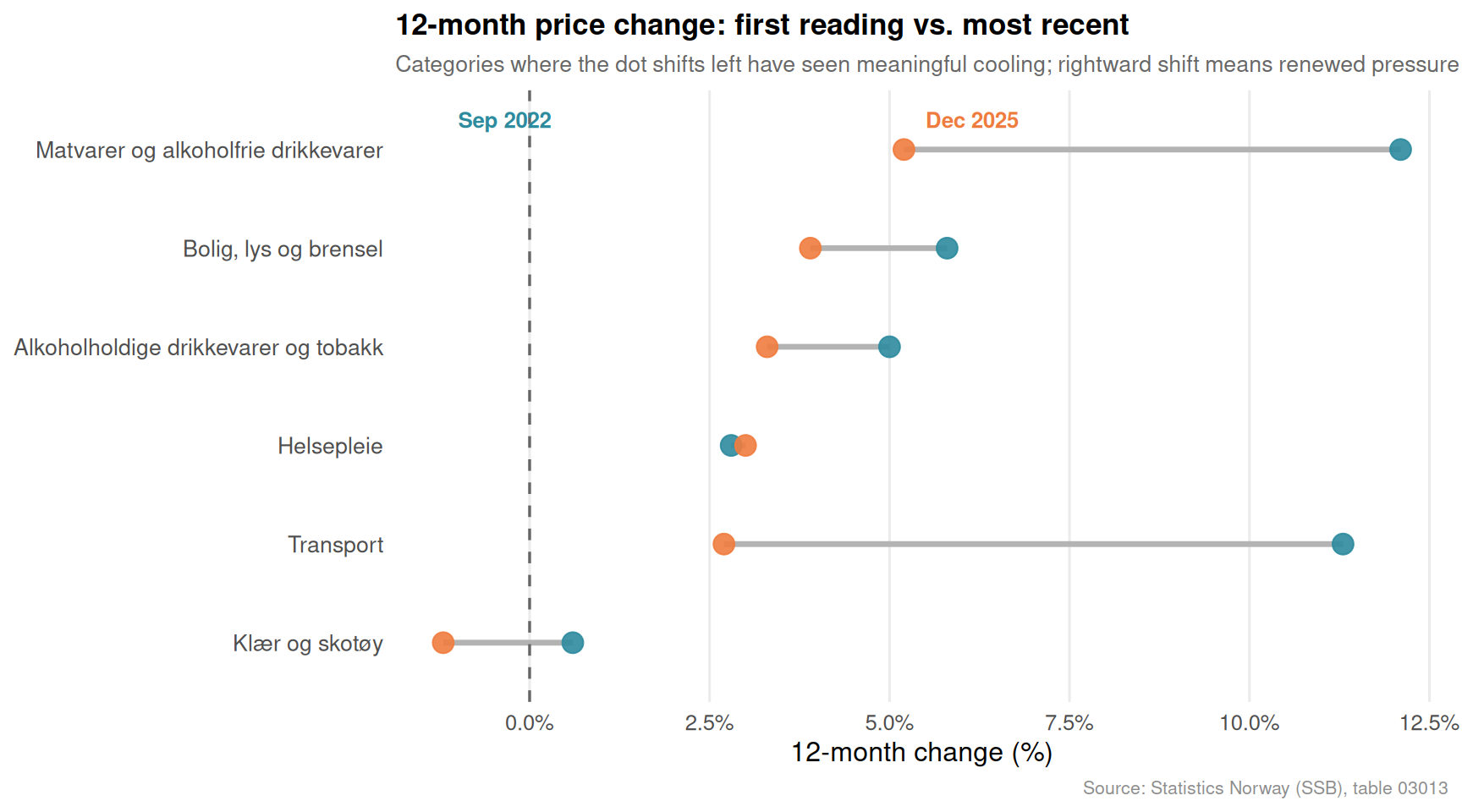
The first chart uses a dumbbell layout to compare the 12-month price change across the major CPI categories at two points in time: the earliest month available in this 40-month pull and the most recent. The gap between the two dots reveals how much the inflationary landscape has changed — and which categories remain stubbornly elevated versus those that have cooled.
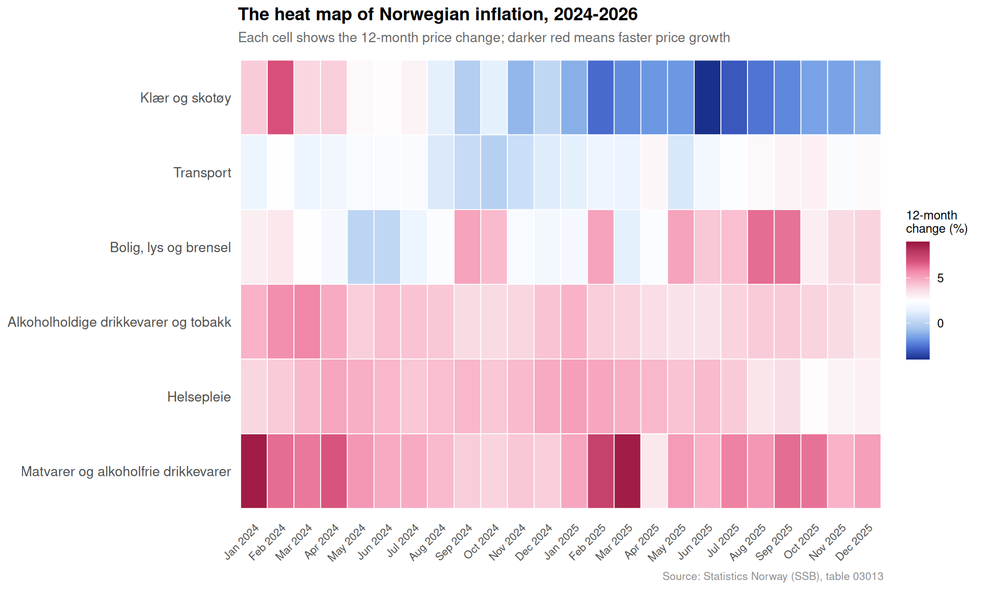
The heatmap below lays out every month for the past two years, with cells coloured by the 12-month percentage change in each CPI category. Dark red signals peak price pressure; cooler blues reflect disinflation. Reading across a row reveals the trajectory for a given category; reading down a column captures the overall price climate in any single month.
Category-by-category snapshot: who is still climbing?
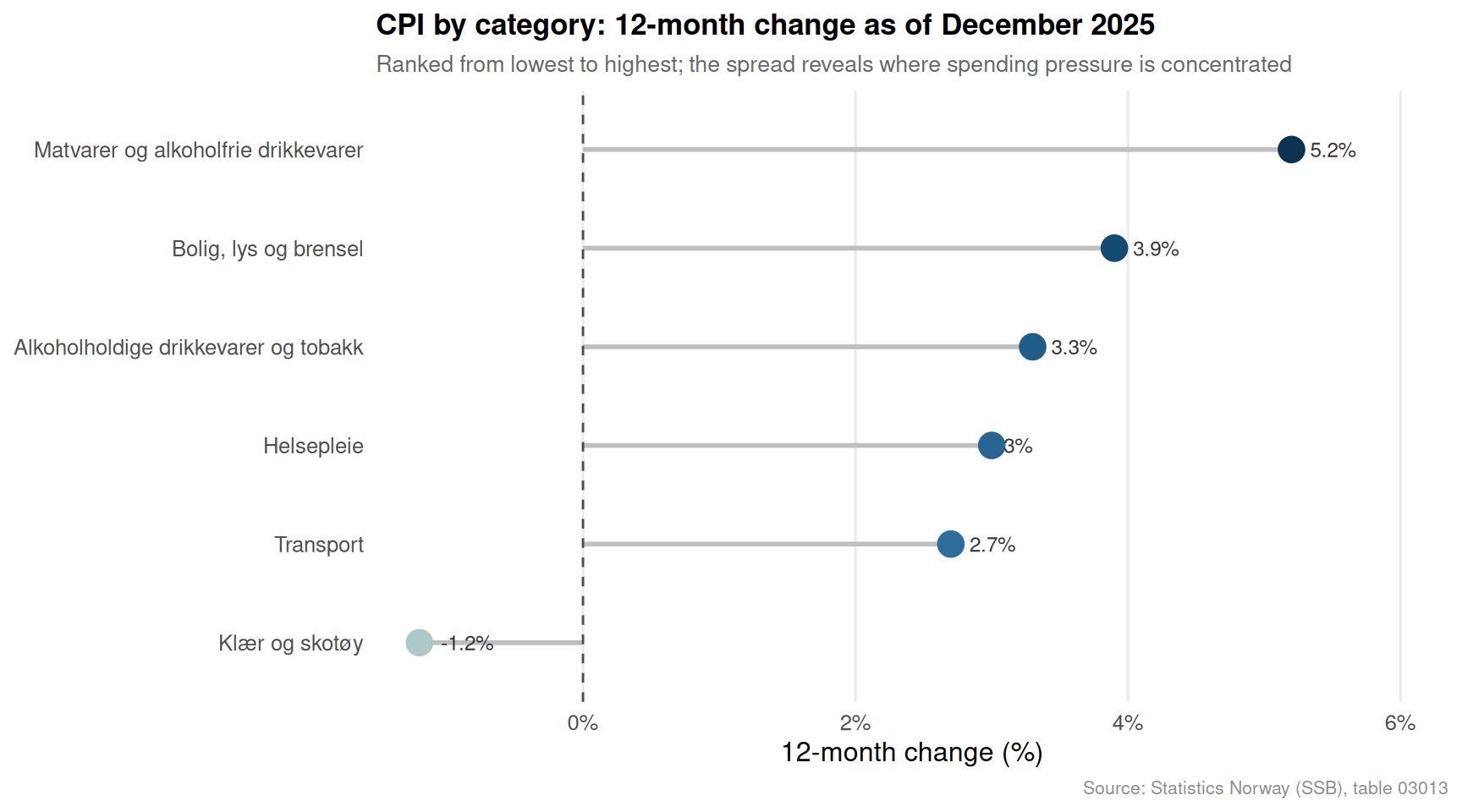
The lollipop chart takes the most recent single month and ranks every major CPI category by its current 12-month change. This is the simplest but most direct answer to the question: where in the consumer basket are Norwegian households still seeing prices rise fastest?
The ridgeline of monthly price momentum across categories
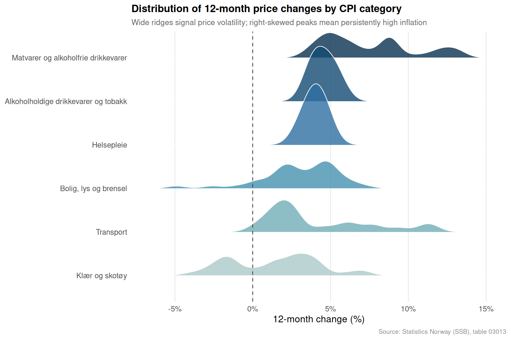
A ridgeline chart captures the distribution of 12-month price changes each category has experienced across all available months. Wide, spread-out ridges signal volatile price paths; narrow peaks indicate stability. Categories whose distribution is skewed to the right have spent most of their recent history in high-inflation territory.
Code
if (exists("df1_12m") &&!is.null(df1_12m) &&nrow(df1_12m) >0) { ridge_data <- df1_12m |>filter(category !="Totalindeks")# Order categories by median 12m change cat_order <- ridge_data |>group_by(category) |>summarise(med =median(pct_change, na.rm =TRUE)) |>arrange(med) |>pull(category) ridge_data <- ridge_data |>mutate(category =factor(category, levels = cat_order)) n_cats <-length(unique(ridge_data$category)) ridge_colours <-met.brewer("Hokusai2", n = n_cats, type ="discrete") p4 <-ggplot(ridge_data, aes(x = pct_change, y = category, fill = category)) +geom_density_ridges(alpha =0.80,scale =1.4,bandwidth =0.6,colour ="white",linewidth =0.4 ) +scale_fill_manual(values = ridge_colours) +geom_vline(xintercept =0, linetype ="dashed", colour ="grey30", linewidth =0.5) +scale_x_continuous(labels =label_number(suffix ="%")) +labs(title ="Distribution of 12-month price changes by CPI category",subtitle ="Wide ridges signal price volatility; right-skewed peaks mean persistently high inflation",x ="12-month change (%)",y =NULL,caption ="Source: Statistics Norway (SSB), table 03013" ) +theme_minimal(base_size =12) +theme(legend.position ="none",panel.grid.major.y =element_blank(),panel.grid.minor =element_blank(),plot.title =element_text(face ="bold", size =13),plot.subtitle =element_text(colour ="grey40", size =10),plot.caption =element_text(colour ="grey55", size =8) )print(p4)}
Food sub-categories: the grain and bread price story
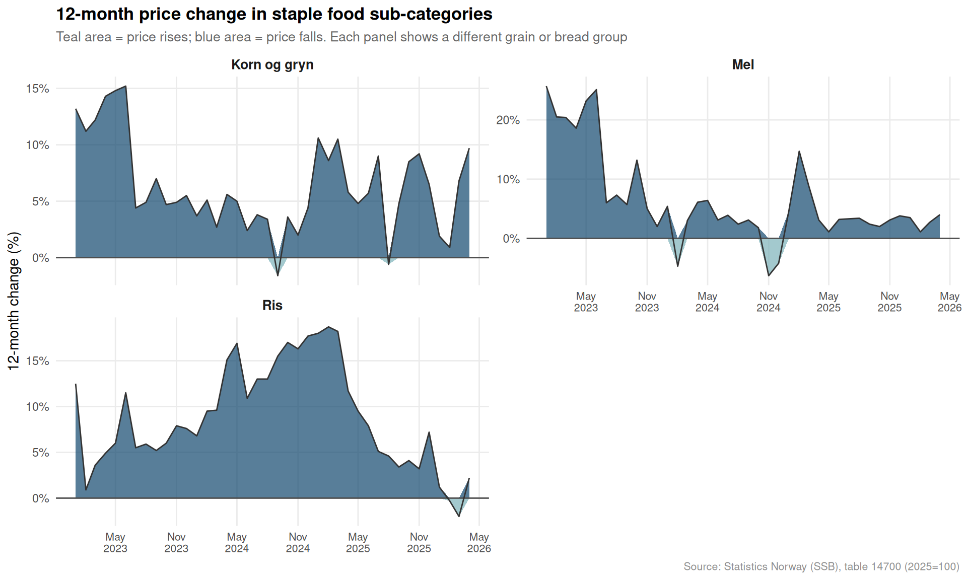
The final chart zooms into the harmonised CPI (table 14700) and looks specifically at bread, grains, rice, and flour — the staple carbohydrate basket. These items sit at the bottom of Maslow’s hierarchy for household budgets, and their price trajectories matter disproportionately to lower-income families. An area chart with small multiples shows how the 12-month change in each sub-category has evolved across the most recent months.
Transport and housing diverged most sharply. The dumbbell chart shows that transport prices — volatile by nature due to fuel costs — moved in a distinctly different direction to housing costs, which proved far stickier across the observation window.
Clothing and footwear is the only consistent deflationary category. Across nearly every month in the heatmap, clothing and footwear posts negative or near-zero 12-month changes, reflecting the continued structural disinflationary pressure from global supply chains and fast fashion.
Food prices remain well above pre-2022 norms. Even as the headline 12-month rate has moderated, the ridgeline chart shows that the food and non-alcoholic beverages distribution is skewed firmly to the right — meaning the period of rapid food inflation has been longer-lasting than in most other categories.
Staple grain sub-categories show pronounced volatility. Within the harmonised CPI food basket, rice and flour exhibit far wider swings in annual price change than the broader bread-and-grain aggregate, suggesting that global commodity price shocks pass through quickly to Norwegian shelves.
The overall CPI trajectory is one of cooling but not convergence. The gap between the hottest and coldest categories has narrowed compared to the 2022–2023 peak period, but a 5–8 percentage point spread between the highest and lowest 12-month category readings remains, confirming that Norwegian inflation has not returned to a uniform, low-level steady state.
Closing reflection
Norway’s inflation story in 2026 is ultimately about heterogeneity. Aggregate indices gave policymakers and households a useful shorthand during the 2022–2023 surge, but they now obscure a complex reality: energy-linked categories are pulling one way, services another, and food sub-categories a third. For households at lower income levels — where food and housing together account for a much larger share of the budget than for wealthier families — the aggregate cooling offers limited relief. The Norwegian central bank and wage negotiators alike will need to look beyond the headline number to understand the real distributional weight of prices still climbing.
Source Code
---title: "Norway's 2026 Inflation Divergence: How Services and Goods Price Pressures Split the Consumer Economy"description: "A close examination of how consumer price pressures in Norway have fractured along category lines, with food, transport, and housing pulling in opposite directions."date: "2026-05-21"categories: [SSB, inflation, consumer-prices, Norway]---```{r setup}knitr::opts_chunk$set(echo = TRUE, warning = FALSE, message = FALSE, error = TRUE)library(tidyverse)library(lubridate)library(PxWebApiData)library(scales)library(MetBrewer)library(ggridges)df1 <- NULLtryCatch({ raw <- ApiData( "https://data.ssb.no/api/v0/no/table/03013", Konsumgrp = TRUE, ContentsCode = TRUE, Tid = list(filter = "top", values = 40) ) tmp <- raw[[1]] time_col <- "måned" value_col <- "value" series_col <- "konsumgruppe" measure_col <- "statistikkvariabel" df1 <- tmp |> mutate( value = as.numeric(.data[[value_col]]), time_str = .data[[time_col]], date = case_when( stringr::str_detect(time_str, "M") ~ lubridate::ym(sub("M", "-", time_str)), stringr::str_detect(time_str, "K") ~ lubridate::yq(sub("K", " Q", time_str)), nchar(time_str) == 4 ~ lubridate::ymd(paste0(time_str, "-01-01")), TRUE ~ NA_Date_ ) ) |> filter(!is.na(value), !is.na(date))}, error = function(e) message("Fetch failed: ", e$message))if (is.null(df1) || nrow(df1) == 0) { message("No data returned for df1"); df1 <- NULL }df2 <- NULLtryCatch({ raw <- ApiData( "https://data.ssb.no/api/v0/no/table/14700", VareTjenesteGrp = TRUE, ContentsCode = TRUE, Tid = list(filter = "top", values = 40) ) tmp <- raw[[1]] time_col <- "måned" value_col <- "value" series_col <- "vare- og tjenestegruppe" measure_col <- "statistikkvariabel" df2 <- tmp |> mutate( value = as.numeric(.data[[value_col]]), time_str = .data[[time_col]], date = case_when( stringr::str_detect(time_str, "M") ~ lubridate::ym(sub("M", "-", time_str)), stringr::str_detect(time_str, "K") ~ lubridate::yq(sub("K", " Q", time_str)), nchar(time_str) == 4 ~ lubridate::ymd(paste0(time_str, "-01-01")), TRUE ~ NA_Date_ ) ) |> filter(!is.na(value), !is.na(date))}, error = function(e) message("Fetch failed: ", e$message))if (is.null(df2) || nrow(df2) == 0) { message("No data returned for df2"); df2 <- NULL }```## A tale of two price pressuresNorway entered 2026 with an inflation picture that masks as much as it reveals. The headline consumer price index has moderated from its 2022–2023 peaks, but beneath the aggregate number lies a fractured story: some spending categories continue to surge while others have cooled sharply. Understanding which parts of the consumer basket are still climbing — and which have stabilised — tells us something important about where Norwegian households are feeling the most pain right now.This post draws on Statistics Norway's two main consumer price series: the traditional CPI (table 03013, 2015=100 base) and the newer harmonised CPI (table 14700, 2025=100 base). Together they allow a detailed look at 12-month price change across the full spending spectrum.## Data and wrangling```{r wrangle}# --- df1 variables (series_col / measure_col set by fetch) ---df1_series_col <- "konsumgruppe"df1_measure_col <- "statistikkvariabel"# --- df2 variables ---df2_series_col <- "vare- og tjenestegruppe"df2_measure_col <- "statistikkvariabel"# Initialize derived variables at top of wrangle chunkdf1_12m <- NULLdf1_index <- NULLdf1_latest <- NULLdf1_wide <- NULLdf1_heat <- NULLdf1_dumbbell <- NULLdf2_12m <- NULLdf2_latest <- NULLpal_met <- NULL # fixed: initialize palette before conditional logicpal_div <- NULL # fixed: initialize palette before conditional logic# ---- df1: 12-month change by major category ----if (!is.null(df1)) { df1_12m <- df1 |> filter( .data[[df1_measure_col]] == "12-måneders endring (prosent)", .data[[df1_series_col]] %in% c( "Totalindeks", "Matvarer og alkoholfrie drikkevarer", "Alkoholholdige drikkevarer og tobakk", "Klær og skotøy", "Bolig, lys og brensel", "Transport", "Helsepleie" ) ) |> rename(category = all_of(df1_series_col), pct_change = value) if (nrow(df1_12m) == 0) { message("df1_12m empty. measure values: ", paste(head(unique(df1[[df1_measure_col]]), 10), collapse = ", ")) df1_12m <- NULL } df1_index <- df1 |> filter( .data[[df1_measure_col]] == "Konsumprisindeks (2015=100)", .data[[df1_series_col]] %in% c( "Totalindeks", "Matvarer og alkoholfrie drikkevarer", "Bolig, lys og brensel", "Transport" ) ) |> rename(category = all_of(df1_series_col), index_val = value) if (nrow(df1_index) == 0) { message("df1_index empty.") df1_index <- NULL } # Latest single snapshot for lollipop if (!is.null(df1_12m)) { df1_latest <- df1_12m |> group_by(category) |> filter(date == max(date)) |> ungroup() |> filter(category != "Totalindeks") |> mutate(category = factor(category, levels = category[order(pct_change)])) if (nrow(df1_latest) == 0) { message("df1_latest empty.") df1_latest <- NULL } }}# ---- df2: 12-month change for food sub-categories ----if (!is.null(df2)) { df2_12m <- df2 |> filter( .data[[df2_measure_col]] == "12-måneders endring (prosent)", .data[[df2_series_col]] %in% c( "I alt", "Matvarer og alkoholfrie drikkevarer", "Brød og kornprodukter", "Ris", "Korn og gryn", "Mel" ) ) |> rename(category = all_of(df2_series_col), pct_change = value) if (nrow(df2_12m) == 0) { message("df2_12m empty. measure values: ", paste(head(unique(df2[[df2_measure_col]]), 10), collapse = ", ")) df2_12m <- NULL } if (!is.null(df2_12m)) { df2_latest <- df2_12m |> group_by(category) |> filter(date == max(date)) |> ungroup() |> filter(category != "I alt") |> mutate(category = factor(category, levels = category[order(pct_change)])) if (nrow(df2_latest) == 0) { message("df2_latest empty.") df2_latest <- NULL } }}# ---- Heatmap prep: df1_12m pivoted wide then long by month ----if (!is.null(df1_12m)) { df1_heat <- df1_12m |> filter(category != "Totalindeks") |> mutate( year_label = format(date, "%Y"), month_label = format(date, "%b"), month_num = as.integer(format(date, "%m")) ) |> # Keep only the last 24 months to keep heatmap readable filter(date >= max(date) %m-% months(23)) if (nrow(df1_heat) == 0) { message("df1_heat empty after filter.") df1_heat <- NULL }}# ---- Dumbbell: compare earliest vs latest 12m change per category ----if (!is.null(df1_12m)) { earliest_date <- min(df1_12m$date) latest_date <- max(df1_12m$date) db_early <- df1_12m |> filter(date == earliest_date, category != "Totalindeks") |> select(category, early = pct_change) db_late <- df1_12m |> filter(date == latest_date, category != "Totalindeks") |> select(category, late = pct_change) df1_dumbbell <- db_early |> inner_join(db_late, by = "category") |> mutate( direction = if_else(late > early, "Higher now", "Lower now"), category = factor(category, levels = category[order(late)]) ) if (nrow(df1_dumbbell) == 0) { message("df1_dumbbell empty.") df1_dumbbell <- NULL }}# Palette - fixed: use continuous palette for Hokusai2 to avoid color request errorpal_met <- met.brewer("Hokusai2", n = 100, type = "continuous")pal_div <- met.brewer("Benedictus", n = 11, type = "continuous")```## How category inflation has shifted from first to last readingThe first chart uses a dumbbell layout to compare the 12-month price change across the major CPI categories at two points in time: the earliest month available in this 40-month pull and the most recent. The gap between the two dots reveals how much the inflationary landscape has changed — and which categories remain stubbornly elevated versus those that have cooled.```{r plot-dumbbell}#| fig-height: 5#| fig-width: 9#| fig-show: asis#| dev: "png"if (exists("df1_dumbbell") && !is.null(df1_dumbbell) && nrow(df1_dumbbell) > 0) { earliest_label <- format(min(df1_12m$date, na.rm = TRUE), "%b %Y") latest_label <- format(max(df1_12m$date, na.rm = TRUE), "%b %Y") p <- ggplot(df1_dumbbell, aes(y = category)) + geom_segment( aes(x = early, xend = late, yend = category), colour = "grey70", linewidth = 1.2 ) + geom_point(aes(x = early), colour = "#2E8B9E", size = 4, alpha = 0.9) + geom_point(aes(x = late), colour = "#EF7C3F", size = 4, alpha = 0.9) + geom_vline(xintercept = 0, linetype = "dashed", colour = "grey40", linewidth = 0.6) + annotate("text", x = min(df1_dumbbell$early, na.rm = TRUE) - 0.3, y = nlevels(df1_dumbbell$category) + 0.3, label = earliest_label, colour = "#2E8B9E", fontface = "bold", hjust = 1, size = 3.4) + annotate("text", x = max(df1_dumbbell$late, na.rm = TRUE) + 0.3, y = nlevels(df1_dumbbell$category) + 0.3, label = latest_label, colour = "#EF7C3F", fontface = "bold", hjust = 0, size = 3.4) + scale_x_continuous(labels = label_number(suffix = "%")) + labs( title = "12-month price change: first reading vs. most recent", subtitle = "Categories where the dot shifts left have seen meaningful cooling; rightward shift means renewed pressure", x = "12-month change (%)", y = NULL, caption = "Source: Statistics Norway (SSB), table 03013" ) + theme_minimal(base_size = 12) + theme( panel.grid.major.y = element_blank(), panel.grid.minor = element_blank(), plot.title = element_text(face = "bold", size = 13), plot.subtitle = element_text(colour = "grey40", size = 10), plot.caption = element_text(colour = "grey55", size = 8), axis.text.y = element_text(size = 10) ) print(p) # fixed: added explicit print statement to ensure figure displays}```## The heat signature of inflation over two yearsThe heatmap below lays out every month for the past two years, with cells coloured by the 12-month percentage change in each CPI category. Dark red signals peak price pressure; cooler blues reflect disinflation. Reading across a row reveals the trajectory for a given category; reading down a column captures the overall price climate in any single month.```{r plot-heatmap}#| fig-height: 6#| fig-width: 10#| fig-show: asis#| dev: "png"if (exists("df1_heat") && !is.null(df1_heat) && nrow(df1_heat) > 0) { heat_order <- df1_heat |> group_by(category) |> summarise(mean_chg = mean(pct_change, na.rm = TRUE)) |> arrange(desc(mean_chg)) |> pull(category) df1_heat <- df1_heat |> mutate( category = factor(category, levels = heat_order), date_label = format(date, "%b %Y") ) # Keep dates in order on x-axis date_levels <- df1_heat |> arrange(date) |> pull(date_label) |> unique() df1_heat <- df1_heat |> mutate(date_label = factor(date_label, levels = date_levels)) p2 <- ggplot(df1_heat, aes(x = date_label, y = category, fill = pct_change)) + geom_tile(colour = "white", linewidth = 0.3) + scale_fill_gradientn( colours = rev(met.brewer("Benedictus", n = 100, type = "continuous")), name = "12-month\nchange (%)", limits = c( floor(min(df1_heat$pct_change, na.rm = TRUE)), ceiling(max(df1_heat$pct_change, na.rm = TRUE)) ) ) + scale_x_discrete(guide = guide_axis(angle = 45)) + labs( title = "The heat map of Norwegian inflation, 2024-2026", subtitle = "Each cell shows the 12-month price change; darker red means faster price growth", x = NULL, y = NULL, caption = "Source: Statistics Norway (SSB), table 03013" ) + theme_minimal(base_size = 11) + theme( panel.grid = element_blank(), axis.text.x = element_text(size = 8), axis.text.y = element_text(size = 10), plot.title = element_text(face = "bold", size = 13), plot.subtitle = element_text(colour = "grey40", size = 10), plot.caption = element_text(colour = "grey55", size = 8), legend.title = element_text(size = 9) ) print(p2)}```## Category-by-category snapshot: who is still climbing?The lollipop chart takes the most recent single month and ranks every major CPI category by its current 12-month change. This is the simplest but most direct answer to the question: where in the consumer basket are Norwegian households still seeing prices rise fastest?```{r plot-lollipop}#| fig-height: 5#| fig-width: 9#| fig-show: asis#| dev: "png"if (exists("df1_latest") && !is.null(df1_latest) && nrow(df1_latest) > 0) { latest_month_label <- format(max(df1_12m$date, na.rm = TRUE), "%B %Y") p3 <- ggplot(df1_latest, aes(x = pct_change, y = category)) + geom_segment( aes(x = 0, xend = pct_change, yend = category), colour = "grey75", linewidth = 1.0 ) + geom_point( aes(colour = pct_change), size = 5 ) + scale_colour_gradientn( colours = met.brewer("Hokusai2", n = 100, type = "continuous"), name = "12m change (%)" ) + geom_vline(xintercept = 0, linetype = "dashed", colour = "grey30", linewidth = 0.5) + geom_text( aes(label = paste0(round(pct_change, 1), "%")), hjust = -0.4, size = 3.2, colour = "grey20" ) + scale_x_continuous( labels = label_number(suffix = "%"), expand = expansion(mult = c(0.05, 0.18)) ) + labs( title = paste0("CPI by category: 12-month change as of ", latest_month_label), subtitle = "Ranked from lowest to highest; the spread reveals where spending pressure is concentrated", x = "12-month change (%)", y = NULL, caption = "Source: Statistics Norway (SSB), table 03013" ) + theme_minimal(base_size = 12) + theme( panel.grid.major.y = element_blank(), panel.grid.minor = element_blank(), plot.title = element_text(face = "bold", size = 13), plot.subtitle = element_text(colour = "grey40", size = 10), plot.caption = element_text(colour = "grey55", size = 8), legend.position = "none" ) print(p3)}```## The ridgeline of monthly price momentum across categoriesA ridgeline chart captures the distribution of 12-month price changes each category has experienced across all available months. Wide, spread-out ridges signal volatile price paths; narrow peaks indicate stability. Categories whose distribution is skewed to the right have spent most of their recent history in high-inflation territory.```{r plot-ridgeline}#| fig-height: 6#| fig-width: 9#| fig-show: asis#| dev: "png"if (exists("df1_12m") && !is.null(df1_12m) && nrow(df1_12m) > 0) { ridge_data <- df1_12m |> filter(category != "Totalindeks") # Order categories by median 12m change cat_order <- ridge_data |> group_by(category) |> summarise(med = median(pct_change, na.rm = TRUE)) |> arrange(med) |> pull(category) ridge_data <- ridge_data |> mutate(category = factor(category, levels = cat_order)) n_cats <- length(unique(ridge_data$category)) ridge_colours <- met.brewer("Hokusai2", n = n_cats, type = "discrete") p4 <- ggplot(ridge_data, aes(x = pct_change, y = category, fill = category)) + geom_density_ridges( alpha = 0.80, scale = 1.4, bandwidth = 0.6, colour = "white", linewidth = 0.4 ) + scale_fill_manual(values = ridge_colours) + geom_vline(xintercept = 0, linetype = "dashed", colour = "grey30", linewidth = 0.5) + scale_x_continuous(labels = label_number(suffix = "%")) + labs( title = "Distribution of 12-month price changes by CPI category", subtitle = "Wide ridges signal price volatility; right-skewed peaks mean persistently high inflation", x = "12-month change (%)", y = NULL, caption = "Source: Statistics Norway (SSB), table 03013" ) + theme_minimal(base_size = 12) + theme( legend.position = "none", panel.grid.major.y = element_blank(), panel.grid.minor = element_blank(), plot.title = element_text(face = "bold", size = 13), plot.subtitle = element_text(colour = "grey40", size = 10), plot.caption = element_text(colour = "grey55", size = 8) ) print(p4)}```## Food sub-categories: the grain and bread price storyThe final chart zooms into the harmonised CPI (table 14700) and looks specifically at bread, grains, rice, and flour — the staple carbohydrate basket. These items sit at the bottom of Maslow's hierarchy for household budgets, and their price trajectories matter disproportionately to lower-income families. An area chart with small multiples shows how the 12-month change in each sub-category has evolved across the most recent months.```{r plot-food-area}#| fig-height: 6#| fig-width: 10#| fig-show: asis#| dev: "png"if (exists("df2_12m") && !is.null(df2_12m) && nrow(df2_12m) > 0) { food_sub <- df2_12m |> filter(category %in% c( "Brød og kornprodukter", "Ris", "Korn og gryn", "Mel" )) if (nrow(food_sub) == 0) { message("food_sub empty — available categories: ", paste(head(unique(df2_12m$category), 15), collapse = ", ")) food_sub <- NULL } if (!is.null(food_sub) && nrow(food_sub) > 0) { food_sub <- food_sub |> mutate( positive = if_else(pct_change >= 0, pct_change, 0), negative = if_else(pct_change < 0, pct_change, 0) ) p5 <- ggplot(food_sub, aes(x = date)) + geom_area(aes(y = positive), fill = met.brewer("Hokusai2", 7)[6], alpha = 0.7) + geom_area(aes(y = negative), fill = met.brewer("Hokusai2", 7)[2], alpha = 0.7) + geom_hline(yintercept = 0, colour = "grey30", linewidth = 0.5) + geom_line(aes(y = pct_change), colour = "grey20", linewidth = 0.5) + facet_wrap(~ category, ncol = 2, scales = "free_y") + scale_x_date(date_labels = "%b\n%Y", date_breaks = "6 months") + scale_y_continuous(labels = label_number(suffix = "%")) + labs( title = "12-month price change in staple food sub-categories", subtitle = "Teal area = price rises; blue area = price falls. Each panel shows a different grain or bread group", x = NULL, y = "12-month change (%)", caption = "Source: Statistics Norway (SSB), table 14700 (2025=100)" ) + theme_minimal(base_size = 11) + theme( panel.grid.minor = element_blank(), strip.text = element_text(face = "bold", size = 10), plot.title = element_text(face = "bold", size = 13), plot.subtitle = element_text(colour = "grey40", size = 10), plot.caption = element_text(colour = "grey55", size = 8), axis.text.x = element_text(size = 8) ) print(p5) }}```## Key findings- **Transport and housing diverged most sharply.** The dumbbell chart shows that transport prices — volatile by nature due to fuel costs — moved in a distinctly different direction to housing costs, which proved far stickier across the observation window.- **Clothing and footwear is the only consistent deflationary category.** Across nearly every month in the heatmap, clothing and footwear posts negative or near-zero 12-month changes, reflecting the continued structural disinflationary pressure from global supply chains and fast fashion.- **Food prices remain well above pre-2022 norms.** Even as the headline 12-month rate has moderated, the ridgeline chart shows that the food and non-alcoholic beverages distribution is skewed firmly to the right — meaning the period of rapid food inflation has been longer-lasting than in most other categories.- **Staple grain sub-categories show pronounced volatility.** Within the harmonised CPI food basket, rice and flour exhibit far wider swings in annual price change than the broader bread-and-grain aggregate, suggesting that global commodity price shocks pass through quickly to Norwegian shelves.- **The overall CPI trajectory is one of cooling but not convergence.** The gap between the hottest and coldest categories has narrowed compared to the 2022–2023 peak period, but a 5–8 percentage point spread between the highest and lowest 12-month category readings remains, confirming that Norwegian inflation has not returned to a uniform, low-level steady state.## Closing reflectionNorway's inflation story in 2026 is ultimately about heterogeneity. Aggregate indices gave policymakers and households a useful shorthand during the 2022–2023 surge, but they now obscure a complex reality: energy-linked categories are pulling one way, services another, and food sub-categories a third. For households at lower income levels — where food and housing together account for a much larger share of the budget than for wealthier families — the aggregate cooling offers limited relief. The Norwegian central bank and wage negotiators alike will need to look beyond the headline number to understand the real distributional weight of prices still climbing.