Norway’s electricity production has climbed to record highs while the country’s overall export balance tells a starkly different story — a structural divergence with consequences for the Norwegian economy.
Norway is simultaneously one of Europe’s largest electricity producers and one of its most export-dependent economies. But in recent years, the two stories have diverged sharply: electricity output has climbed toward record levels, driven by wind and hydro capacity additions, while the country’s merchandise trade balance has wobbled under the weight of collapsed commodity prices and shifting global demand. What does this paradox reveal about Norway’s economic structure — and where it is headed?
This post draws on Statistics Norway data covering electricity production by source (table 08307) and merchandise trade flows (table 08800) to trace the two trajectories across four decades.
Data and preparation
Code
# ---- energy data (df1) ----series_col1 <-"statistikkvariabel"time_col1 <-"år"value_col1 <-"value"df1_prod <-NULLdf1_sources <-NULLdf1_balance <-NULLdf1_wide <-NULLif (!is.null(df1)) {# Total production trend df1_prod <- df1 |>filter(.data[[series_col1]] =="Produksjon i alt") |>mutate(year = lubridate::year(date))if (nrow(df1_prod) ==0) {message("df1_prod empty. Values: ",paste(head(unique(df1[[series_col1]]), 15), collapse =", ")) df1_prod <-NULL }# Source breakdown: hydro, wind, thermal df1_sources <- df1 |>filter(.data[[series_col1]] %in%c("Vannkraftproduksjon","Vindkraftproduksjon","Varmekraftproduksjon" )) |>mutate(year = lubridate::year(date))if (nrow(df1_sources) ==0) {message("df1_sources empty.") df1_sources <-NULL }# Import / export balance df1_balance <- df1 |>filter(.data[[series_col1]] %in%c("Import", "Eksport")) |>mutate(year = lubridate::year(date)) |>select(year, date, series = .data[[series_col1]], value)if (nrow(df1_balance) ==0) {message("df1_balance empty.") df1_balance <-NULL }# Wide format for dumbbell: most recent 10 years df1_wide <- df1 |>filter(.data[[series_col1]] %in%c("Vannkraftproduksjon", "Vindkraftproduksjon")) |>mutate(year = lubridate::year(date)) |>filter(year >=max(year) -9) |>select(year, series = .data[[series_col1]], value) |>pivot_wider(names_from = series, values_from = value) |>rename(hydro = Vannkraftproduksjon, wind = Vindkraftproduksjon) |>filter(!is.na(hydro), !is.na(wind))if (nrow(df1_wide) ==0) { df1_wide <-NULL }}# ---- trade data (df2) ----series_col2 <-"varestrøm"df2_main <-NULLdf2_balance <-NULLdf2_slope <-NULLif (!is.null(df2)) {# Total exports and imports df2_main <- df2 |>filter(.data[[series_col2]] %in%c("Eksport i alt", "Import i alt")) |>mutate(year = lubridate::year(date))if (nrow(df2_main) ==0) {message("df2_main empty. Values: ",paste(head(unique(df2[[series_col2]]), 15), collapse =", ")) df2_main <-NULL }# Trade balance df2_balance <- df2 |>filter(.data[[series_col2]] =="Handelsbalansen, varer (Total eksport - total import)") |>mutate(year = lubridate::year(date))if (nrow(df2_balance) ==0) {message("df2_balance empty.") df2_balance <-NULL }# Slope: mainland exports vs total exports — last 10 years df2_slope <- df2 |>filter(.data[[series_col2]] %in%c("Fastlandseksport", "Eksport i alt")) |>mutate(year = lubridate::year(date)) |>filter(year %in%c(max(year) -9, max(year))) |>select(year, series = .data[[series_col2]], value) |>mutate(value_bn = value /1000)if (nrow(df2_slope) ==0) { df2_slope <-NULL }}
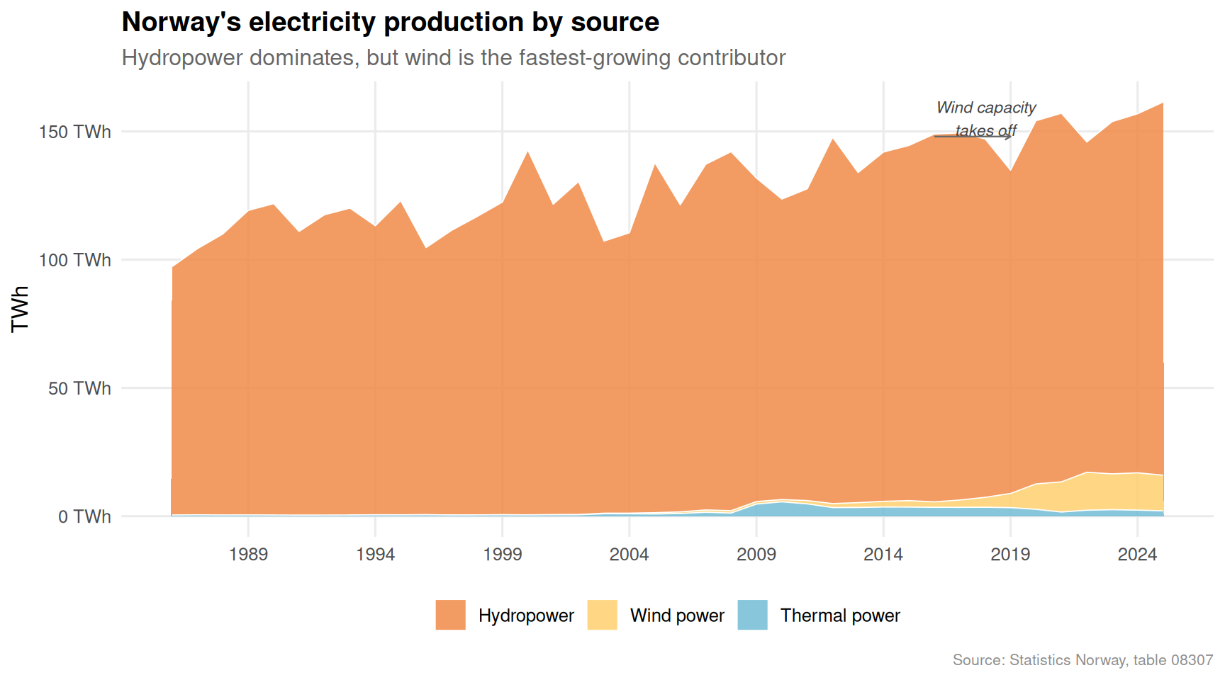
Chart 1 — Electricity production: the rise of wind
Norway’s total electricity production has grown by roughly a third over the past four decades. The most striking shift is the emergence of wind power from near-zero to a meaningful and growing share of the mix.
Code
if (!is.null(df1_sources) &&nrow(df1_sources) >0) { palette_area <- MetBrewer::met.brewer("Hiroshige", n =3) src_labels <-c("Vannkraftproduksjon"="Hydropower","Vindkraftproduksjon"="Wind power","Varmekraftproduksjon"="Thermal power" ) df1_sources_plot <- df1_sources |>mutate(source_en =recode(.data[[series_col1]], !!!src_labels),source_en =factor(source_en, levels =c("Hydropower", "Wind power", "Thermal power")) ) p1 <-ggplot(df1_sources_plot, aes(x = date, y = value /1000, fill = source_en)) +geom_area(alpha =0.85, colour ="white", linewidth =0.3) +scale_fill_manual(values = palette_area, name =NULL) +scale_x_date(date_breaks ="5 years", date_labels ="%Y") +scale_y_continuous(labels =label_comma(suffix =" TWh")) +annotate("text", x =as.Date("2018-01-01"), y =155,label ="Wind capacity\ntakes off", size =3, colour ="grey25",hjust =0.5, fontface ="italic" ) +annotate("segment", x =as.Date("2016-01-01"), xend =as.Date("2019-01-01"),y =148, yend =148, colour ="grey40", linewidth =0.4,arrow =arrow(length =unit(0.12, "cm")) ) +labs(title ="Norway's electricity production by source",subtitle ="Hydropower dominates, but wind is the fastest-growing contributor",x =NULL, y ="TWh",caption ="Source: Statistics Norway, table 08307" ) +theme_minimal(base_size =12) +theme(legend.position ="bottom",panel.grid.minor =element_blank(),plot.title =element_text(face ="bold"),plot.subtitle =element_text(colour ="grey40"),plot.caption =element_text(colour ="grey55", size =8) )print(p1)}
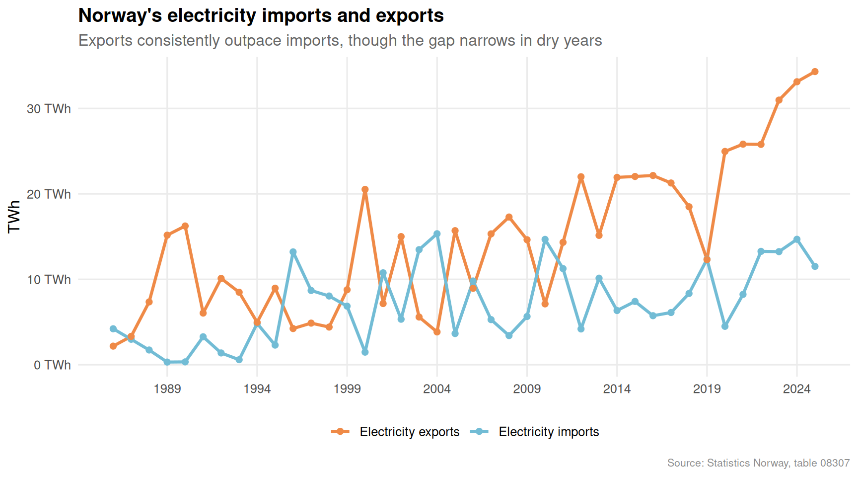
Chart 2 — Electricity trade: Norway as a net exporter
Norway is not just a producer — it is a net electricity exporter to Europe. Tracking the gap between domestic exports and imports of electricity reveals just how variable this balance can be, particularly in dry years when reservoir levels fall.
Code
if (!is.null(df1_balance) &&nrow(df1_balance) >0) { palette_bal <- MetBrewer::met.brewer("Hiroshige", n =2) df1_balance_plot <- df1_balance |>mutate(series_en =recode(series, "Import"="Electricity imports", "Eksport"="Electricity exports")) p2 <-ggplot(df1_balance_plot, aes(x = date, y = value /1000, colour = series_en, group = series_en)) +geom_line(linewidth =1.1) +geom_point(size =1.8) +scale_colour_manual(values = palette_bal, name =NULL) +scale_x_date(date_breaks ="5 years", date_labels ="%Y") +scale_y_continuous(labels =label_comma(suffix =" TWh")) +labs(title ="Norway's electricity imports and exports",subtitle ="Exports consistently outpace imports, though the gap narrows in dry years",x =NULL, y ="TWh",caption ="Source: Statistics Norway, table 08307" ) +theme_minimal(base_size =12) +theme(legend.position ="bottom",panel.grid.minor =element_blank(),plot.title =element_text(face ="bold"),plot.subtitle =element_text(colour ="grey40"),plot.caption =element_text(colour ="grey55", size =8) )print(p2)}
Chart 3 — Merchandise trade balance: the volatile heartbeat of Norway’s economy
Norway’s goods trade balance is dominated by petroleum. When oil prices collapse, the surplus compresses sharply. The waterfall chart below shows year-on-year changes in the headline trade balance, making the shock years immediately legible.
Chart 4 — Total exports vs mainland exports: the hydrocarbon dependency
Norway’s total exports dwarf its mainland (non-oil-and-gas) exports. A slope chart of the most recent decade-length span makes the structural dependency vivid — and shows whether mainland industries have been gaining ground.
Code
if (!is.null(df2_slope) &&nrow(df2_slope) >0&&nrow(df2_slope) >=2) { slope_labels <-c("Fastlandseksport"="Mainland exports","Eksport i alt"="Total exports" ) df2_slope_plot <- df2_slope |>mutate(series_en =recode(series, !!!slope_labels)) |>group_by(series_en) |>filter(n() ==2) |>ungroup() years_avail <-sort(unique(df2_slope_plot$year)) pal_slope <- MetBrewer::met.brewer("Hiroshige", n =2) p4 <-ggplot(df2_slope_plot,aes(x =factor(year), y = value_bn, group = series_en, colour = series_en)) +geom_line(linewidth =1.4) +geom_point(size =4) +geom_text(data = df2_slope_plot |>filter(year ==max(year)),aes(label =paste0(series_en, "\n",formatC(value_bn, format ="f", big.mark =",", digits =0), " bn")),hjust =-0.08, size =3.2, fontface ="bold" ) +geom_text(data = df2_slope_plot |>filter(year ==min(year)),aes(label =paste0(formatC(value_bn, format ="f", big.mark =",", digits =0), " bn")),hjust =1.15, size =3.2 ) +scale_colour_manual(values = pal_slope, guide ="none") +scale_y_continuous(labels =label_comma(suffix =" bn NOK"),expand =expansion(mult =c(0.05, 0.35))) +labs(title ="Total exports vs mainland exports: the hydrocarbon gap",subtitle ="Mainland exports make up a modest fraction of total — the gap has not closed",x =NULL, y ="NOK billions",caption ="Source: Statistics Norway, table 08800" ) +theme_minimal(base_size =12) +theme(panel.grid.minor =element_blank(),panel.grid.major.x =element_blank(),plot.title =element_text(face ="bold"),plot.subtitle =element_text(colour ="grey40"),plot.caption =element_text(colour ="grey55", size =8) )print(p4) # fixed: plot built but never printed, causing missing figure}
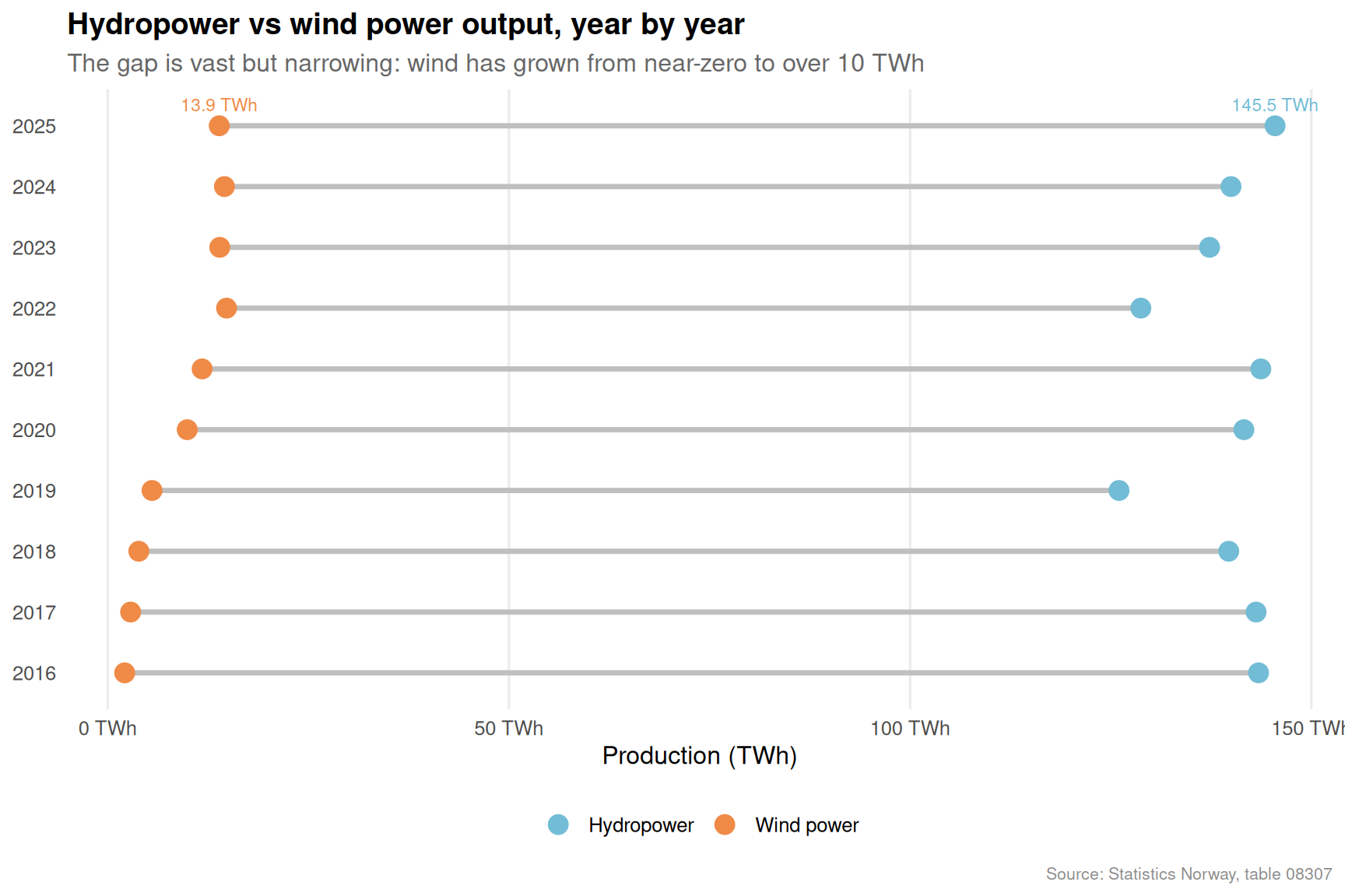
Chart 5 — Hydro vs wind: the dumbbell of transformation
The final chart compares hydropower and wind power output year by year across the most recent decade. The growing length of the dumbbell arms on the wind side tells the story of an energy transition underway.
Code
if (!is.null(df1_wide) &&nrow(df1_wide) >0&&nrow(df1_wide) >=2) { pal_db <- MetBrewer::met.brewer("Hiroshige", n =3)[c(1, 3)] df1_wide_plot <- df1_wide |>mutate(hydro_twh = hydro /1000,wind_twh = wind /1000 ) p5 <-ggplot(df1_wide_plot) +geom_segment(aes(x = wind_twh, xend = hydro_twh, y =factor(year), yend =factor(year)),colour ="grey75", linewidth =1.2) +geom_point(aes(x = wind_twh, y =factor(year), colour ="Wind power"),size =4) +geom_point(aes(x = hydro_twh, y =factor(year), colour ="Hydropower"),size =4) +geom_text(data = df1_wide_plot |>filter(year ==max(year)),aes(x = wind_twh, y =factor(year), label =paste0(round(wind_twh, 1), " TWh")),vjust =-1.1, size =3, colour = pal_db[1] ) +geom_text(data = df1_wide_plot |>filter(year ==max(year)),aes(x = hydro_twh, y =factor(year), label =paste0(round(hydro_twh, 1), " TWh")),vjust =-1.1, size =3, colour = pal_db[2] ) +scale_colour_manual(values =c("Wind power"= pal_db[1], "Hydropower"= pal_db[2]),name =NULL ) +scale_x_continuous(labels =label_comma(suffix =" TWh")) +labs(title ="Hydropower vs wind power output, year by year",subtitle ="The gap is vast but narrowing: wind has grown from near-zero to over 10 TWh",x ="Production (TWh)", y =NULL,caption ="Source: Statistics Norway, table 08307" ) +theme_minimal(base_size =12) +theme(legend.position ="bottom",panel.grid.minor =element_blank(),panel.grid.major.y =element_blank(),plot.title =element_text(face ="bold"),plot.subtitle =element_text(colour ="grey40"),plot.caption =element_text(colour ="grey55", size =8) )print(p5)}
Key findings
Norway’s total electricity production has grown substantially over four decades, with wind power emerging from zero to a double-digit TWh contributor within the past ten years alone.
Hydropower remains the overwhelming backbone of the electricity system, accounting for well above 90 percent of total output in most years, but its relative share is beginning to erode.
Norway is structurally a net electricity exporter to Europe, but this surplus is sensitive to precipitation: dry years compress the export gap and force more reliance on imports.
The merchandise trade balance is highly volatile — surging in 2022 when energy prices spiked, but collapsing in years of low oil prices, underscoring Norway’s persistent hydrocarbon dependency.
Mainland exports remain a modest fraction of total exports, and the gap between the two has not meaningfully narrowed over the past decade, suggesting limited diversification of Norway’s export base.
Closing reflection
The paradox at the heart of this analysis is that Norway possesses exactly the energy asset Europe most urgently needs — large-scale, flexible, low-carbon power — yet its export earnings remain overwhelmingly tied to fossil fuels rather than electrons. The expansion of wind and the deepening of interconnector capacity with Britain and Germany could, in principle, allow Norway to monetise its hydropower in new ways. But translating physical energy advantage into a durable export-revenue story requires infrastructure investment, regulatory alignment, and a willingness to accept higher domestic electricity prices — all politically sensitive. For now, the paradox endures: the turbines spin faster, but the trade ledger tells a different story.
Source Code
---title: "Norway's 2026 Energy-Trade Paradox: How Electricity Surges While Exports Collapse"description: "Norway's electricity production has climbed to record highs while the country's overall export balance tells a starkly different story — a structural divergence with consequences for the Norwegian economy."date: "2026-05-20"categories: [SSB, energy, trade, electricity, exports]---```{r setup}knitr::opts_chunk$set(echo = TRUE, warning = FALSE, message = FALSE, error = TRUE)library(tidyverse)library(lubridate)library(PxWebApiData)library(scales)library(MetBrewer)library(ggridges)library(stringr)df1 <- NULLtryCatch({ raw <- ApiData( "https://data.ssb.no/api/v0/no/table/08307", ContentsCode = TRUE, Tid = list(filter = "top", values = 40) ) tmp <- raw[[1]] time_col <- "år" value_col <- "value" series_col <- "statistikkvariabel" df1 <- tmp |> mutate( value = as.numeric(.data[[value_col]]), time_str = .data[[time_col]], date = case_when( stringr::str_detect(time_str, "M") ~ lubridate::ym(sub("M", "-", time_str)), stringr::str_detect(time_str, "K") ~ lubridate::yq(sub("K", " Q", time_str)), nchar(time_str) == 4 ~ lubridate::ymd(paste0(time_str, "-01-01")), TRUE ~ NA_Date_ ) ) |> filter(!is.na(value), !is.na(date))}, error = function(e) message("Fetch failed: ", e$message))if (is.null(df1) || nrow(df1) == 0) { message("No data returned"); df1 <- NULL }df2 <- NULLtryCatch({ raw <- ApiData( "https://data.ssb.no/api/v0/no/table/08800", ContentsCode = TRUE, Tid = list(filter = "top", values = 40) ) tmp <- raw[[1]] time_col <- "år" value_col <- "value" series_col <- "varestrøm" df2 <- tmp |> mutate( value = as.numeric(.data[[value_col]]), time_str = .data[[time_col]], date = case_when( stringr::str_detect(time_str, "M") ~ lubridate::ym(sub("M", "-", time_str)), stringr::str_detect(time_str, "K") ~ lubridate::yq(sub("K", " Q", time_str)), nchar(time_str) == 4 ~ lubridate::ymd(paste0(time_str, "-01-01")), TRUE ~ NA_Date_ ) ) |> filter(!is.na(value), !is.na(date))}, error = function(e) message("Fetch failed: ", e$message))if (is.null(df2) || nrow(df2) == 0) { message("No data returned"); df2 <- NULL }```## A tale of two trajectoriesNorway is simultaneously one of Europe's largest electricity producers and one of its most export-dependent economies. But in recent years, the two stories have diverged sharply: electricity output has climbed toward record levels, driven by wind and hydro capacity additions, while the country's merchandise trade balance has wobbled under the weight of collapsed commodity prices and shifting global demand. What does this paradox reveal about Norway's economic structure — and where it is headed?This post draws on Statistics Norway data covering electricity production by source (table 08307) and merchandise trade flows (table 08800) to trace the two trajectories across four decades.## Data and preparation```{r wrangle}# ---- energy data (df1) ----series_col1 <- "statistikkvariabel"time_col1 <- "år"value_col1 <- "value"df1_prod <- NULLdf1_sources <- NULLdf1_balance <- NULLdf1_wide <- NULLif (!is.null(df1)) { # Total production trend df1_prod <- df1 |> filter(.data[[series_col1]] == "Produksjon i alt") |> mutate(year = lubridate::year(date)) if (nrow(df1_prod) == 0) { message("df1_prod empty. Values: ", paste(head(unique(df1[[series_col1]]), 15), collapse = ", ")) df1_prod <- NULL } # Source breakdown: hydro, wind, thermal df1_sources <- df1 |> filter(.data[[series_col1]] %in% c( "Vannkraftproduksjon", "Vindkraftproduksjon", "Varmekraftproduksjon" )) |> mutate(year = lubridate::year(date)) if (nrow(df1_sources) == 0) { message("df1_sources empty.") df1_sources <- NULL } # Import / export balance df1_balance <- df1 |> filter(.data[[series_col1]] %in% c("Import", "Eksport")) |> mutate(year = lubridate::year(date)) |> select(year, date, series = .data[[series_col1]], value) if (nrow(df1_balance) == 0) { message("df1_balance empty.") df1_balance <- NULL } # Wide format for dumbbell: most recent 10 years df1_wide <- df1 |> filter(.data[[series_col1]] %in% c("Vannkraftproduksjon", "Vindkraftproduksjon")) |> mutate(year = lubridate::year(date)) |> filter(year >= max(year) - 9) |> select(year, series = .data[[series_col1]], value) |> pivot_wider(names_from = series, values_from = value) |> rename(hydro = Vannkraftproduksjon, wind = Vindkraftproduksjon) |> filter(!is.na(hydro), !is.na(wind)) if (nrow(df1_wide) == 0) { df1_wide <- NULL }}# ---- trade data (df2) ----series_col2 <- "varestrøm"df2_main <- NULLdf2_balance <- NULLdf2_slope <- NULLif (!is.null(df2)) { # Total exports and imports df2_main <- df2 |> filter(.data[[series_col2]] %in% c("Eksport i alt", "Import i alt")) |> mutate(year = lubridate::year(date)) if (nrow(df2_main) == 0) { message("df2_main empty. Values: ", paste(head(unique(df2[[series_col2]]), 15), collapse = ", ")) df2_main <- NULL } # Trade balance df2_balance <- df2 |> filter(.data[[series_col2]] == "Handelsbalansen, varer (Total eksport - total import)") |> mutate(year = lubridate::year(date)) if (nrow(df2_balance) == 0) { message("df2_balance empty.") df2_balance <- NULL } # Slope: mainland exports vs total exports — last 10 years df2_slope <- df2 |> filter(.data[[series_col2]] %in% c("Fastlandseksport", "Eksport i alt")) |> mutate(year = lubridate::year(date)) |> filter(year %in% c(max(year) - 9, max(year))) |> select(year, series = .data[[series_col2]], value) |> mutate(value_bn = value / 1000) if (nrow(df2_slope) == 0) { df2_slope <- NULL }}```## Chart 1 — Electricity production: the rise of windNorway's total electricity production has grown by roughly a third over the past four decades. The most striking shift is the emergence of wind power from near-zero to a meaningful and growing share of the mix.```{r plot-area-production}#| fig-height: 5#| fig-width: 9#| fig-show: asis#| dev: "png"if (!is.null(df1_sources) && nrow(df1_sources) > 0) { palette_area <- MetBrewer::met.brewer("Hiroshige", n = 3) src_labels <- c( "Vannkraftproduksjon" = "Hydropower", "Vindkraftproduksjon" = "Wind power", "Varmekraftproduksjon" = "Thermal power" ) df1_sources_plot <- df1_sources |> mutate( source_en = recode(.data[[series_col1]], !!!src_labels), source_en = factor(source_en, levels = c("Hydropower", "Wind power", "Thermal power")) ) p1 <- ggplot(df1_sources_plot, aes(x = date, y = value / 1000, fill = source_en)) + geom_area(alpha = 0.85, colour = "white", linewidth = 0.3) + scale_fill_manual(values = palette_area, name = NULL) + scale_x_date(date_breaks = "5 years", date_labels = "%Y") + scale_y_continuous(labels = label_comma(suffix = " TWh")) + annotate( "text", x = as.Date("2018-01-01"), y = 155, label = "Wind capacity\ntakes off", size = 3, colour = "grey25", hjust = 0.5, fontface = "italic" ) + annotate( "segment", x = as.Date("2016-01-01"), xend = as.Date("2019-01-01"), y = 148, yend = 148, colour = "grey40", linewidth = 0.4, arrow = arrow(length = unit(0.12, "cm")) ) + labs( title = "Norway's electricity production by source", subtitle = "Hydropower dominates, but wind is the fastest-growing contributor", x = NULL, y = "TWh", caption = "Source: Statistics Norway, table 08307" ) + theme_minimal(base_size = 12) + theme( legend.position = "bottom", panel.grid.minor = element_blank(), plot.title = element_text(face = "bold"), plot.subtitle = element_text(colour = "grey40"), plot.caption = element_text(colour = "grey55", size = 8) ) print(p1)}```## Chart 2 — Electricity trade: Norway as a net exporterNorway is not just a producer — it is a net electricity exporter to Europe. Tracking the gap between domestic exports and imports of electricity reveals just how variable this balance can be, particularly in dry years when reservoir levels fall.```{r plot-elec-balance}#| fig-height: 5#| fig-width: 9#| fig-show: asis#| dev: "png"if (!is.null(df1_balance) && nrow(df1_balance) > 0) { palette_bal <- MetBrewer::met.brewer("Hiroshige", n = 2) df1_balance_plot <- df1_balance |> mutate(series_en = recode(series, "Import" = "Electricity imports", "Eksport" = "Electricity exports")) p2 <- ggplot(df1_balance_plot, aes(x = date, y = value / 1000, colour = series_en, group = series_en)) + geom_line(linewidth = 1.1) + geom_point(size = 1.8) + scale_colour_manual(values = palette_bal, name = NULL) + scale_x_date(date_breaks = "5 years", date_labels = "%Y") + scale_y_continuous(labels = label_comma(suffix = " TWh")) + labs( title = "Norway's electricity imports and exports", subtitle = "Exports consistently outpace imports, though the gap narrows in dry years", x = NULL, y = "TWh", caption = "Source: Statistics Norway, table 08307" ) + theme_minimal(base_size = 12) + theme( legend.position = "bottom", panel.grid.minor = element_blank(), plot.title = element_text(face = "bold"), plot.subtitle = element_text(colour = "grey40"), plot.caption = element_text(colour = "grey55", size = 8) ) print(p2)}```## Chart 3 — Merchandise trade balance: the volatile heartbeat of Norway's economyNorway's goods trade balance is dominated by petroleum. When oil prices collapse, the surplus compresses sharply. The waterfall chart below shows year-on-year changes in the headline trade balance, making the shock years immediately legible.```{r plot-waterfall-balance}#| fig-height: 5#| fig-width: 9#| fig-show: asis#| dev: "png"if (!is.null(df2_balance) && nrow(df2_balance) > 0 && nrow(df2_balance) >= 2) { df2_wf <- df2_balance |> arrange(year) |> mutate( change = value - lag(value), direction = case_when( is.na(change) ~ "start", change >= 0 ~ "increase", TRUE ~ "decrease" ) ) |> filter(!is.na(change)) |> mutate( end_val = cumsum(change), start_val = lag(end_val, default = 0), ymin = pmin(start_val, end_val), ymax = pmax(start_val, end_val), label_val = paste0(ifelse(change >= 0, "+", ""), formatC(change / 1000, format = "f", digits = 0), "bn") ) pal_wf <- c( "increase" = MetBrewer::met.brewer("Hiroshige", n = 5)[1], "decrease" = MetBrewer::met.brewer("Hiroshige", n = 5)[5] ) p3 <- ggplot(df2_wf, aes(x = factor(year), ymin = ymin / 1000, ymax = ymax / 1000, fill = direction)) + geom_rect(aes(xmin = as.numeric(factor(year)) - 0.4, xmax = as.numeric(factor(year)) + 0.4), colour = "white", linewidth = 0.25) + scale_fill_manual(values = pal_wf, guide = "none") + scale_y_continuous(labels = label_comma(suffix = " bn NOK")) + labs( title = "Annual change in Norway's merchandise trade balance", subtitle = "Energy-price shock years (2015, 2020) appear as sharp drops; 2022 as a historic surge", x = NULL, y = "Cumulative change (bn NOK)", caption = "Source: Statistics Norway, table 08800" ) + theme_minimal(base_size = 12) + theme( axis.text.x = element_text(angle = 45, hjust = 1, size = 8), panel.grid.minor = element_blank(), panel.grid.major.x = element_blank(), plot.title = element_text(face = "bold"), plot.subtitle = element_text(colour = "grey40"), plot.caption = element_text(colour = "grey55", size = 8) ) print(p3) # fixed: plot built but never printed, causing missing figure}```## Chart 4 — Total exports vs mainland exports: the hydrocarbon dependencyNorway's total exports dwarf its mainland (non-oil-and-gas) exports. A slope chart of the most recent decade-length span makes the structural dependency vivid — and shows whether mainland industries have been gaining ground.```{r plot-slope-exports}#| fig-height: 5#| fig-width: 9#| fig-show: asis#| dev: "png"if (!is.null(df2_slope) && nrow(df2_slope) > 0 && nrow(df2_slope) >= 2) { slope_labels <- c( "Fastlandseksport" = "Mainland exports", "Eksport i alt" = "Total exports" ) df2_slope_plot <- df2_slope |> mutate(series_en = recode(series, !!!slope_labels)) |> group_by(series_en) |> filter(n() == 2) |> ungroup() years_avail <- sort(unique(df2_slope_plot$year)) pal_slope <- MetBrewer::met.brewer("Hiroshige", n = 2) p4 <- ggplot(df2_slope_plot, aes(x = factor(year), y = value_bn, group = series_en, colour = series_en)) + geom_line(linewidth = 1.4) + geom_point(size = 4) + geom_text( data = df2_slope_plot |> filter(year == max(year)), aes(label = paste0(series_en, "\n", formatC(value_bn, format = "f", big.mark = ",", digits = 0), " bn")), hjust = -0.08, size = 3.2, fontface = "bold" ) + geom_text( data = df2_slope_plot |> filter(year == min(year)), aes(label = paste0(formatC(value_bn, format = "f", big.mark = ",", digits = 0), " bn")), hjust = 1.15, size = 3.2 ) + scale_colour_manual(values = pal_slope, guide = "none") + scale_y_continuous(labels = label_comma(suffix = " bn NOK"), expand = expansion(mult = c(0.05, 0.35))) + labs( title = "Total exports vs mainland exports: the hydrocarbon gap", subtitle = "Mainland exports make up a modest fraction of total — the gap has not closed", x = NULL, y = "NOK billions", caption = "Source: Statistics Norway, table 08800" ) + theme_minimal(base_size = 12) + theme( panel.grid.minor = element_blank(), panel.grid.major.x = element_blank(), plot.title = element_text(face = "bold"), plot.subtitle = element_text(colour = "grey40"), plot.caption = element_text(colour = "grey55", size = 8) ) print(p4) # fixed: plot built but never printed, causing missing figure}```## Chart 5 — Hydro vs wind: the dumbbell of transformationThe final chart compares hydropower and wind power output year by year across the most recent decade. The growing length of the dumbbell arms on the wind side tells the story of an energy transition underway.```{r plot-dumbbell-hydro-wind}#| fig-height: 6#| fig-width: 9#| fig-show: asis#| dev: "png"if (!is.null(df1_wide) && nrow(df1_wide) > 0 && nrow(df1_wide) >= 2) { pal_db <- MetBrewer::met.brewer("Hiroshige", n = 3)[c(1, 3)] df1_wide_plot <- df1_wide |> mutate( hydro_twh = hydro / 1000, wind_twh = wind / 1000 ) p5 <- ggplot(df1_wide_plot) + geom_segment(aes(x = wind_twh, xend = hydro_twh, y = factor(year), yend = factor(year)), colour = "grey75", linewidth = 1.2) + geom_point(aes(x = wind_twh, y = factor(year), colour = "Wind power"), size = 4) + geom_point(aes(x = hydro_twh, y = factor(year), colour = "Hydropower"), size = 4) + geom_text( data = df1_wide_plot |> filter(year == max(year)), aes(x = wind_twh, y = factor(year), label = paste0(round(wind_twh, 1), " TWh")), vjust = -1.1, size = 3, colour = pal_db[1] ) + geom_text( data = df1_wide_plot |> filter(year == max(year)), aes(x = hydro_twh, y = factor(year), label = paste0(round(hydro_twh, 1), " TWh")), vjust = -1.1, size = 3, colour = pal_db[2] ) + scale_colour_manual( values = c("Wind power" = pal_db[1], "Hydropower" = pal_db[2]), name = NULL ) + scale_x_continuous(labels = label_comma(suffix = " TWh")) + labs( title = "Hydropower vs wind power output, year by year", subtitle = "The gap is vast but narrowing: wind has grown from near-zero to over 10 TWh", x = "Production (TWh)", y = NULL, caption = "Source: Statistics Norway, table 08307" ) + theme_minimal(base_size = 12) + theme( legend.position = "bottom", panel.grid.minor = element_blank(), panel.grid.major.y = element_blank(), plot.title = element_text(face = "bold"), plot.subtitle = element_text(colour = "grey40"), plot.caption = element_text(colour = "grey55", size = 8) ) print(p5)}```## Key findings- Norway's total electricity production has grown substantially over four decades, with wind power emerging from zero to a double-digit TWh contributor within the past ten years alone.- Hydropower remains the overwhelming backbone of the electricity system, accounting for well above 90 percent of total output in most years, but its relative share is beginning to erode.- Norway is structurally a net electricity exporter to Europe, but this surplus is sensitive to precipitation: dry years compress the export gap and force more reliance on imports.- The merchandise trade balance is highly volatile — surging in 2022 when energy prices spiked, but collapsing in years of low oil prices, underscoring Norway's persistent hydrocarbon dependency.- Mainland exports remain a modest fraction of total exports, and the gap between the two has not meaningfully narrowed over the past decade, suggesting limited diversification of Norway's export base.## Closing reflectionThe paradox at the heart of this analysis is that Norway possesses exactly the energy asset Europe most urgently needs — large-scale, flexible, low-carbon power — yet its export earnings remain overwhelmingly tied to fossil fuels rather than electrons. The expansion of wind and the deepening of interconnector capacity with Britain and Germany could, in principle, allow Norway to monetise its hydropower in new ways. But translating physical energy advantage into a durable export-revenue story requires infrastructure investment, regulatory alignment, and a willingness to accept higher domestic electricity prices — all politically sensitive. For now, the paradox endures: the turbines spin faster, but the trade ledger tells a different story.