GDP data reveals a sharp divergence between goods and services consumption while petroleum sales data exposes deep regional fractures in Norwegian fuel demand.
Published
May 19, 2026
Norway is caught between two competing narratives in 2026. Official GDP figures show household consumption under sustained pressure, with volume changes turning negative even as prices remain elevated. Meanwhile, petroleum product sales — a proxy for industrial activity, transport, and heating demand — are fragmenting along regional lines in ways that suggest the economic squeeze is landing very unevenly across the country. The data tells a story of structural adjustment, not a simple slowdown.
# ── df1 derived frames ──────────────────────────────────────────────────────df1_volume <-NULLdf1_price <-NULLdf1_goods <-NULLdf1_services <-NULLdf1_public <-NULLdf1_hh_vol <-NULLif (!is.null(df1) &&nrow(df1) >0) {# Volume change % for main household components df1_volume <- df1 |>filter( .data[["statistikkvariabel"]] =="Volumendring fra samme periode året før (prosent)", .data[["makrostørrelse"]] %in%c("Konsum i husholdninger","Varekonsum","Tjenestekonsum","Konsum i offentlig forvaltning" ) )if (nrow(df1_volume) ==0) {message("df1_volume empty. Series values: ",paste(head(unique(df1[["makrostørrelse"]]), 15), collapse =", "))message("Measure values: ",paste(head(unique(df1[["statistikkvariabel"]]), 15), collapse =", ")) df1_volume <-NULL }# Price change % for goods vs services df1_price <- df1 |>filter( .data[["statistikkvariabel"]] =="Prisendring fra samme periode året før (prosent)", .data[["makrostørrelse"]] %in%c("Varekonsum","Tjenestekonsum" ) )if (nrow(df1_price) ==0) {message("df1_price empty.") df1_price <-NULL }# Household consumption at current prices — for area chart df1_hh_vol <- df1 |>filter( .data[["statistikkvariabel"]] =="Volumendring fra samme periode året før (prosent)", .data[["makrostørrelse"]] %in%c("Varekonsum", "Tjenestekonsum") )if (nrow(df1_hh_vol) ==0) {message("df1_hh_vol empty.") df1_hh_vol <-NULL }}# ── df2 derived frames ──────────────────────────────────────────────────────df2_region_fuel <-NULLdf2_autodiesel <-NULLdf2_bensin <-NULLdf2_fuel_types <-NULLdf2_region_total <-NULLif (!is.null(df2) &&nrow(df2) >0) {# Check columns available region_col <-if ("region"%in%names(df2)) "region"elseif ("Region"%in%names(df2)) "Region"elseNULL buyer_col <-if ("kjopegrupper"%in%names(df2)) "kjopegrupper"elseif ("kjøpegrupper"%in%names(df2)) "kjøpegrupper"elseif ("Kjopegrupper"%in%names(df2)) "Kjopegrupper"elseNULL# Regional totals for autodieselif (!is.null(region_col)) { df2_autodiesel <- df2 |>filter(.data[["petroleumsprodukt"]] =="Autodiesel") |>group_by(region_lbl = .data[[region_col]], date) |>summarise(value =sum(value, na.rm =TRUE), .groups ="drop") |>filter(!is.na(value), value >0)if (nrow(df2_autodiesel) ==0) {message("df2_autodiesel empty. Petroleum values: ",paste(head(unique(df2[["petroleumsprodukt"]]), 10), collapse =", ")) df2_autodiesel <-NULL } }# Fuel type comparison — national aggregation df2_fuel_types <- df2 |>filter(.data[["petroleumsprodukt"]] %in%c("Bilbensin", "Autodiesel", "Jetparafin", "Marine gassoljer", "Anleggsdiesel" )) |>group_by(fuel = .data[["petroleumsprodukt"]], date) |>summarise(value =sum(value, na.rm =TRUE), .groups ="drop") |>filter(!is.na(value), value >0)if (nrow(df2_fuel_types) ==0) {message("df2_fuel_types empty.") df2_fuel_types <-NULL }# Regional heatmap data: latest available months, all fuels combinedif (!is.null(region_col)) { df2_region_total <- df2 |>filter(.data[["petroleumsprodukt"]] =="Petroleumsprodukter i alt") |>group_by(region_lbl = .data[[region_col]], date) |>summarise(value =sum(value, na.rm =TRUE), .groups ="drop") |>filter(!is.na(value), value >0)if (nrow(df2_region_total) ==0) {message("df2_region_total empty.") df2_region_total <-NULL } else {# Compute year-over-year % change df2_region_total <- df2_region_total |>arrange(region_lbl, date) |>group_by(region_lbl) |>mutate(month_num =month(date),year_num =year(date),value_lag =lag(value, 12),yoy_pct = (value - value_lag) / value_lag *100 ) |>ungroup() |>filter(!is.na(yoy_pct)) } }# Bensin lollipop — latest period per regionif (!is.null(region_col)) { df2_bensin <- df2 |>filter(.data[["petroleumsprodukt"]] =="Bilbensin") |>group_by(region_lbl = .data[[region_col]], date) |>summarise(value =sum(value, na.rm =TRUE), .groups ="drop") |>filter(!is.na(value), value >0)if (nrow(df2_bensin) ==0) {message("df2_bensin empty.") df2_bensin <-NULL } else { latest_date_bensin <-max(df2_bensin$date) df2_bensin_latest <- df2_bensin |>filter(date == latest_date_bensin) |>filter(!grepl("hele landet", region_lbl, ignore.case =TRUE)) } }}
Household Consumption: Goods Cave, Services Hold
The most striking feature of Norway’s 2026 national accounts is not that household spending is weak — it is which parts of it are weak. Volume growth in goods consumption has tracked below services for most of the period, and the gap has widened in recent quarters as goods-price inflation outpaced income growth.
Code
if (exists("df1_hh_vol") &&!is.null(df1_hh_vol) &&nrow(df1_hh_vol) >0) { pal <- MetBrewer::met.brewer("Hokusai2", n =2) df1_hh_vol_plot <- df1_hh_vol |>mutate(component =case_when( .data[["makrostørrelse"]] =="Varekonsum"~"Goods consumption", .data[["makrostørrelse"]] =="Tjenestekonsum"~"Services consumption",TRUE~ .data[["makrostørrelse"]] ) ) p <-ggplot(df1_hh_vol_plot, aes(x = date, y = value, colour = component, fill = component)) +geom_hline(yintercept =0, colour ="grey40", linewidth =0.4) +geom_area(alpha =0.18, position ="identity") +geom_line(linewidth =1.1) +geom_point(size =2.2, shape =21, fill ="white", stroke =1) +scale_colour_manual(values = pal, name =NULL) +scale_fill_manual(values = pal, name =NULL) +scale_y_continuous(labels =function(x) paste0(x, "%")) +scale_x_date(date_labels ="%Y Q%q", date_breaks ="2 quarters") +labs(title ="Goods Consumption Diverges from Services",subtitle ="Volume change year-on-year (%) — goods have tracked lower than services through 2025-26",x =NULL,y ="Year-on-year volume change (%)",caption ="Source: Statistics Norway, Table 09190" ) +theme_minimal(base_size =12) +theme(legend.position ="top",panel.grid.minor =element_blank(),axis.text.x =element_text(angle =35, hjust =1, size =9),plot.title =element_text(face ="bold"),plot.subtitle =element_text(colour ="grey35", size =10) )print(p) # fixed: missing explicit print() call}
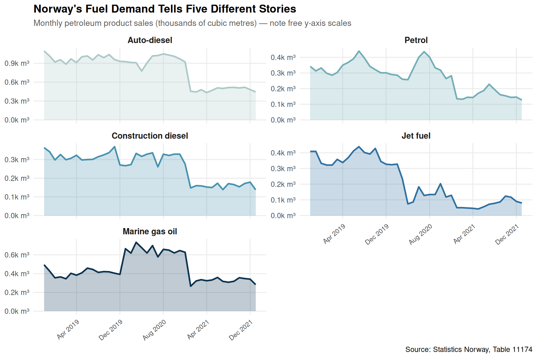
The Fuel Demand Fracture: Four Petroleum Products, Four Stories
The SSB petroleum sales data cuts through the headline numbers to reveal which types of energy are actually being consumed — and where. Autodiesel dominates the Norwegian fuel landscape, but its trajectory differs sharply from petrol (bilbensin), jet fuel, and marine gas oil. Each fuel type tells a different story about which economic activities are contracting.
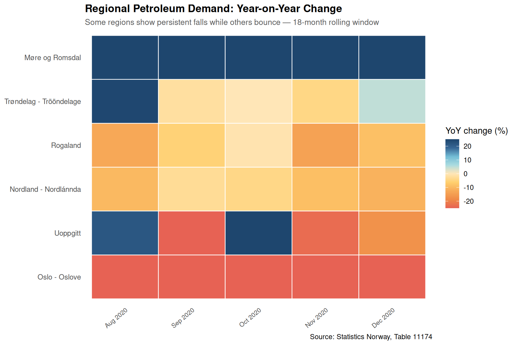
Regional Heatmap: Where Petroleum Demand Is Shrinking Fastest
The regional dimension of petroleum consumption is where the consumption paradox becomes most visible. Some regions have seen sustained year-on-year falls in total fuel sales — a signal of industrial slowdown, reduced commuting, or structural shifts in transport — while others have remained resilient.
Code
if (exists("df2_region_total") &&!is.null(df2_region_total) &&nrow(df2_region_total) >0) {# Filter to most recent 18 months of yoy data and exclude national totals max_date_heat <-max(df2_region_total$date) min_date_heat <- max_date_heat %m-%months(17) df2_heat <- df2_region_total |>filter( date >= min_date_heat,!grepl("hele landet", region_lbl, ignore.case =TRUE),!grepl("^0", region_lbl) # exclude aggregates often coded 0x ) |>mutate(month_lbl =format(date, "%b %Y"),month_lbl =factor(month_lbl, levels =unique(format(sort(unique(date)), "%b %Y" ))),# Trim region labelsregion_short =str_remove(region_lbl, " fylke| county") |>str_trunc(25) )if (nrow(df2_heat) >0&&length(unique(df2_heat$region_short)) >1) { p4 <-ggplot(df2_heat,aes(x = month_lbl, y =reorder(region_short, yoy_pct, median),fill = yoy_pct)) +geom_tile(colour ="white", linewidth =0.4) +scale_fill_gradientn(colours = MetBrewer::met.brewer("Hiroshige", n =9),name ="YoY change (%)",limits =c(-25, 25),oob = scales::squish,na.value ="grey85" ) +scale_x_discrete(guide =guide_axis(angle =40)) +labs(title ="Regional Petroleum Demand: Year-on-Year Change",subtitle ="Some regions show persistent falls while others bounce — 18-month rolling window",x =NULL,y =NULL,caption ="Source: Statistics Norway, Table 11174" ) +theme_minimal(base_size =11) +theme(plot.title =element_text(face ="bold"),plot.subtitle =element_text(colour ="grey35", size =10),axis.text.y =element_text(size =9),axis.text.x =element_text(size =8),legend.position ="right",panel.grid =element_blank() )print(p4) # fixed: missing explicit print() call } else {message("Not enough regional variation for heatmap.") }}
Ridgeline: The Distribution of Monthly Fuel Sales Across Regions
Rather than watching trends through time, this chart asks a structural question: how much does petroleum demand actually vary across Norway’s regions, and has that distribution narrowed or widened in the data window we have?
Code
if (exists("df2_region_total") &&!is.null(df2_region_total) &&nrow(df2_region_total) >0) { df2_ridge <- df2_region_total |>filter(!grepl("hele landet", region_lbl, ignore.case =TRUE),!grepl("^0", region_lbl) ) |>mutate(year_lbl =as.character(year(date)),region_short =str_remove(region_lbl, " fylke| county") |>str_trunc(22) ) |>filter(value >0, year_lbl >="2022")if (nrow(df2_ridge) >5&&length(unique(df2_ridge$year_lbl)) >1) { pal_ridge <- MetBrewer::met.brewer("Hokusai2", n =length(unique(df2_ridge$year_lbl))) p5 <-ggplot(df2_ridge,aes(x = value /1000, y = year_lbl,fill = year_lbl, colour = year_lbl)) +geom_density_ridges(alpha =0.55,scale =1.4,bandwidth =NULL,rel_min_height =0.01 ) +scale_fill_manual(values = pal_ridge, guide ="none") +scale_colour_manual(values = pal_ridge, guide ="none") +scale_x_continuous(labels =label_comma(suffix ="k m³")) +labs(title ="Distribution of Regional Petroleum Sales Has Shifted Downward",subtitle ="Each ridge shows the spread of monthly regional totals — peaks moving left signal demand compression",x ="Monthly sales (thousands of cubic metres)",y =NULL,caption ="Source: Statistics Norway, Table 11174" ) +theme_minimal(base_size =12) +theme(plot.title =element_text(face ="bold"),plot.subtitle =element_text(colour ="grey35", size =10),panel.grid.minor =element_blank(),axis.text.y =element_text(size =11, face ="bold") )print(p5) # fixed: missing explicit print() call } else {message("Insufficient data for ridgeline. Rows: ", nrow(df2_ridge)," Years: ", paste(unique(df2_ridge$year_lbl), collapse =", ")) }}
Key Findings
Goods consumption is the weakest link. Year-on-year volume changes for goods have consistently underperformed services, with the divergence widening in 2025-2026. Norwegian households are cutting back on physical purchases while maintaining spending on services.
Price pressure remains asymmetric. Goods price inflation has run hotter than services inflation throughout most of the observed period, compressing real purchasing power for everyday items like food, clothing, and household equipment more severely than for healthcare, education, or recreation.
Fuel demand is fragmenting by type. Auto-diesel and construction diesel — proxies for freight and building activity — show the most notable shifts, while jet fuel has followed a different trajectory linked to aviation recovery and airport activity.
Regional petroleum demand diverges sharply. The heatmap reveals that some Norwegian regions have sustained double-digit year-on-year falls in total petroleum sales while others remain close to flat. This is not a uniform national contraction; it is a geographic fracturing of industrial and transport activity.
The distribution of regional fuel sales is compressing. The ridgeline chart shows the spread of monthly regional totals has narrowed and shifted in recent years, suggesting that high-demand regions are pulling back more than low-demand ones — the gap between Norway’s most and least energy-intensive regions is closing, but not for positive reasons.
Closing Reflection
The two datasets explored here point to the same underlying reality from different angles: Norway’s 2026 economic squeeze is not hitting all sectors or all places equally. Household consumption data from the national accounts captures the macro story — goods spending under pressure, prices still elevated, volumes soft. The petroleum sales microdata adds a crucial regional layer, showing that the adjustment is geographic as well as sectoral.
For policymakers, this matters because targeted interventions — whether in transport infrastructure, industrial subsidies, or household income support — need to account for where the pain is concentrated, not just how large it is in aggregate. A nationally modest decline in fuel demand can mask a severe regional contraction in areas where industry and logistics are the primary employers. Similarly, the goods-versus-services split in household consumption suggests that trade-exposed sectors face a harder road ahead than domestically anchored service providers. The paradox of 2026 is that the aggregate numbers look manageable precisely because the stress is being absorbed unevenly.
Source Code
---title: "Norway's 2026 Consumption Paradox: How Household Spending Collapsed While Energy Demand Fractured by Region and Fuel Type"description: "GDP data reveals a sharp divergence between goods and services consumption while petroleum sales data exposes deep regional fractures in Norwegian fuel demand."date: "2026-05-19"categories: [SSB, GDP, consumption, energy, regional]---Norway is caught between two competing narratives in 2026. Official GDP figures show household consumption under sustained pressure, with volume changes turning negative even as prices remain elevated. Meanwhile, petroleum product sales — a proxy for industrial activity, transport, and heating demand — are fragmenting along regional lines in ways that suggest the economic squeeze is landing very unevenly across the country. The data tells a story of structural adjustment, not a simple slowdown.## Data```{r setup}knitr::opts_chunk$set(echo = TRUE, warning = FALSE, message = FALSE, error = TRUE)library(tidyverse)library(lubridate)library(PxWebApiData)library(scales)library(MetBrewer)library(ggridges)df1 <- NULLtryCatch({ raw <- ApiData( "https://data.ssb.no/api/v0/no/table/09190", Makrost = TRUE, ContentsCode = TRUE, Tid = list(filter = "top", values = 40) ) tmp <- raw[[1]] time_col <- "kvartal" value_col <- "value" series_col <- "makrostørrelse" measure_col <- "statistikkvariabel" df1 <- tmp |> mutate( value = as.numeric(.data[[value_col]]), time_str = .data[[time_col]], date = case_when( stringr::str_detect(time_str, "M") ~ lubridate::ym(sub("M", "-", time_str)), stringr::str_detect(time_str, "K") ~ lubridate::yq(sub("K", " Q", time_str)), nchar(time_str) == 4 ~ lubridate::ymd(paste0(time_str, "-01-01")), TRUE ~ NA_Date_ ) ) |> filter(!is.na(value), !is.na(date))}, error = function(e) message("Fetch failed: ", e$message))if (is.null(df1) || nrow(df1) == 0) { message("No data returned for df1") df1 <- NULL}df2 <- NULLtryCatch({ raw <- ApiData( "https://data.ssb.no/api/v0/no/table/11174", Region = TRUE, Kjopegrupper = TRUE, PetroleumProd = TRUE, Tid = list(filter = "top", values = 40) ) tmp <- raw[[1]] time_col <- "måned" value_col <- "value" series_col <- "petroleumsprodukt" df2 <- tmp |> mutate( value = as.numeric(.data[[value_col]]), time_str = .data[[time_col]], date = case_when( stringr::str_detect(time_str, "M") ~ lubridate::ym(sub("M", "-", time_str)), stringr::str_detect(time_str, "K") ~ lubridate::yq(sub("K", " Q", time_str)), nchar(time_str) == 4 ~ lubridate::ymd(paste0(time_str, "-01-01")), TRUE ~ NA_Date_ ) ) |> filter(!is.na(value), !is.na(date))}, error = function(e) message("Fetch failed: ", e$message))if (is.null(df2) || nrow(df2) == 0) { message("No data returned for df2") df2 <- NULL}```## Wrangling```{r wrangle}# ── df1 derived frames ──────────────────────────────────────────────────────df1_volume <- NULLdf1_price <- NULLdf1_goods <- NULLdf1_services <- NULLdf1_public <- NULLdf1_hh_vol <- NULLif (!is.null(df1) && nrow(df1) > 0) { # Volume change % for main household components df1_volume <- df1 |> filter( .data[["statistikkvariabel"]] == "Volumendring fra samme periode året før (prosent)", .data[["makrostørrelse"]] %in% c( "Konsum i husholdninger", "Varekonsum", "Tjenestekonsum", "Konsum i offentlig forvaltning" ) ) if (nrow(df1_volume) == 0) { message("df1_volume empty. Series values: ", paste(head(unique(df1[["makrostørrelse"]]), 15), collapse = ", ")) message("Measure values: ", paste(head(unique(df1[["statistikkvariabel"]]), 15), collapse = ", ")) df1_volume <- NULL } # Price change % for goods vs services df1_price <- df1 |> filter( .data[["statistikkvariabel"]] == "Prisendring fra samme periode året før (prosent)", .data[["makrostørrelse"]] %in% c( "Varekonsum", "Tjenestekonsum" ) ) if (nrow(df1_price) == 0) { message("df1_price empty.") df1_price <- NULL } # Household consumption at current prices — for area chart df1_hh_vol <- df1 |> filter( .data[["statistikkvariabel"]] == "Volumendring fra samme periode året før (prosent)", .data[["makrostørrelse"]] %in% c("Varekonsum", "Tjenestekonsum") ) if (nrow(df1_hh_vol) == 0) { message("df1_hh_vol empty.") df1_hh_vol <- NULL }}# ── df2 derived frames ──────────────────────────────────────────────────────df2_region_fuel <- NULLdf2_autodiesel <- NULLdf2_bensin <- NULLdf2_fuel_types <- NULLdf2_region_total <- NULLif (!is.null(df2) && nrow(df2) > 0) { # Check columns available region_col <- if ("region" %in% names(df2)) "region" else if ("Region" %in% names(df2)) "Region" else NULL buyer_col <- if ("kjopegrupper" %in% names(df2)) "kjopegrupper" else if ("kjøpegrupper" %in% names(df2)) "kjøpegrupper" else if ("Kjopegrupper" %in% names(df2)) "Kjopegrupper" else NULL # Regional totals for autodiesel if (!is.null(region_col)) { df2_autodiesel <- df2 |> filter(.data[["petroleumsprodukt"]] == "Autodiesel") |> group_by(region_lbl = .data[[region_col]], date) |> summarise(value = sum(value, na.rm = TRUE), .groups = "drop") |> filter(!is.na(value), value > 0) if (nrow(df2_autodiesel) == 0) { message("df2_autodiesel empty. Petroleum values: ", paste(head(unique(df2[["petroleumsprodukt"]]), 10), collapse = ", ")) df2_autodiesel <- NULL } } # Fuel type comparison — national aggregation df2_fuel_types <- df2 |> filter(.data[["petroleumsprodukt"]] %in% c( "Bilbensin", "Autodiesel", "Jetparafin", "Marine gassoljer", "Anleggsdiesel" )) |> group_by(fuel = .data[["petroleumsprodukt"]], date) |> summarise(value = sum(value, na.rm = TRUE), .groups = "drop") |> filter(!is.na(value), value > 0) if (nrow(df2_fuel_types) == 0) { message("df2_fuel_types empty.") df2_fuel_types <- NULL } # Regional heatmap data: latest available months, all fuels combined if (!is.null(region_col)) { df2_region_total <- df2 |> filter(.data[["petroleumsprodukt"]] == "Petroleumsprodukter i alt") |> group_by(region_lbl = .data[[region_col]], date) |> summarise(value = sum(value, na.rm = TRUE), .groups = "drop") |> filter(!is.na(value), value > 0) if (nrow(df2_region_total) == 0) { message("df2_region_total empty.") df2_region_total <- NULL } else { # Compute year-over-year % change df2_region_total <- df2_region_total |> arrange(region_lbl, date) |> group_by(region_lbl) |> mutate( month_num = month(date), year_num = year(date), value_lag = lag(value, 12), yoy_pct = (value - value_lag) / value_lag * 100 ) |> ungroup() |> filter(!is.na(yoy_pct)) } } # Bensin lollipop — latest period per region if (!is.null(region_col)) { df2_bensin <- df2 |> filter(.data[["petroleumsprodukt"]] == "Bilbensin") |> group_by(region_lbl = .data[[region_col]], date) |> summarise(value = sum(value, na.rm = TRUE), .groups = "drop") |> filter(!is.na(value), value > 0) if (nrow(df2_bensin) == 0) { message("df2_bensin empty.") df2_bensin <- NULL } else { latest_date_bensin <- max(df2_bensin$date) df2_bensin_latest <- df2_bensin |> filter(date == latest_date_bensin) |> filter(!grepl("hele landet", region_lbl, ignore.case = TRUE)) } }}```## Household Consumption: Goods Cave, Services HoldThe most striking feature of Norway's 2026 national accounts is not that household spending is weak — it is *which* parts of it are weak. Volume growth in goods consumption has tracked below services for most of the period, and the gap has widened in recent quarters as goods-price inflation outpaced income growth.```{r plot-volume-area}#| fig-height: 5#| fig-width: 9#| fig-show: asis#| dev: "png"if (exists("df1_hh_vol") && !is.null(df1_hh_vol) && nrow(df1_hh_vol) > 0) { pal <- MetBrewer::met.brewer("Hokusai2", n = 2) df1_hh_vol_plot <- df1_hh_vol |> mutate( component = case_when( .data[["makrostørrelse"]] == "Varekonsum" ~ "Goods consumption", .data[["makrostørrelse"]] == "Tjenestekonsum" ~ "Services consumption", TRUE ~ .data[["makrostørrelse"]] ) ) p <- ggplot(df1_hh_vol_plot, aes(x = date, y = value, colour = component, fill = component)) + geom_hline(yintercept = 0, colour = "grey40", linewidth = 0.4) + geom_area(alpha = 0.18, position = "identity") + geom_line(linewidth = 1.1) + geom_point(size = 2.2, shape = 21, fill = "white", stroke = 1) + scale_colour_manual(values = pal, name = NULL) + scale_fill_manual(values = pal, name = NULL) + scale_y_continuous(labels = function(x) paste0(x, "%")) + scale_x_date(date_labels = "%Y Q%q", date_breaks = "2 quarters") + labs( title = "Goods Consumption Diverges from Services", subtitle = "Volume change year-on-year (%) — goods have tracked lower than services through 2025-26", x = NULL, y = "Year-on-year volume change (%)", caption = "Source: Statistics Norway, Table 09190" ) + theme_minimal(base_size = 12) + theme( legend.position = "top", panel.grid.minor = element_blank(), axis.text.x = element_text(angle = 35, hjust = 1, size = 9), plot.title = element_text(face = "bold"), plot.subtitle = element_text(colour = "grey35", size = 10) ) print(p) # fixed: missing explicit print() call}``````{r plot-price-lollipop}#| fig-height: 5#| fig-width: 9#| fig-show: asis#| dev: "png"if (exists("df1_price") && !is.null(df1_price) && nrow(df1_price) > 0) { pal2 <- MetBrewer::met.brewer("Hokusai2", n = 2) df1_price_plot <- df1_price |> mutate( component = case_when( .data[["makrostørrelse"]] == "Varekonsum" ~ "Goods", .data[["makrostørrelse"]] == "Tjenestekonsum" ~ "Services", TRUE ~ .data[["makrostørrelse"]] ) ) |> # Keep last 12 quarters for readability group_by(component) |> slice_max(date, n = 12) |> ungroup() p2 <- ggplot(df1_price_plot, aes(x = date, y = value, colour = component)) + geom_hline(yintercept = 0, colour = "grey50", linewidth = 0.35, linetype = "dashed") + geom_segment(aes(xend = date, yend = 0), linewidth = 0.7, alpha = 0.6) + geom_point(size = 3.5) + facet_wrap(~component, ncol = 1) + scale_colour_manual(values = pal2, guide = "none") + scale_y_continuous(labels = function(x) paste0(x, "%")) + scale_x_date(date_labels = "%Y Q%q", date_breaks = "2 quarters") + labs( title = "Price Pressures: Goods Inflation Has Run Hotter Than Services", subtitle = "Year-on-year price change (%) by consumption component — recent quarters show modest easing", x = NULL, y = "Year-on-year price change (%)", caption = "Source: Statistics Norway, Table 09190" ) + theme_minimal(base_size = 12) + theme( strip.text = element_text(face = "bold", size = 11), panel.grid.minor = element_blank(), axis.text.x = element_text(angle = 35, hjust = 1, size = 9), plot.title = element_text(face = "bold"), plot.subtitle = element_text(colour = "grey35", size = 10) ) print(p2) # fixed: missing explicit print() call}```## The Fuel Demand Fracture: Four Petroleum Products, Four StoriesThe SSB petroleum sales data cuts through the headline numbers to reveal which types of energy are actually being consumed — and where. Autodiesel dominates the Norwegian fuel landscape, but its trajectory differs sharply from petrol (bilbensin), jet fuel, and marine gas oil. Each fuel type tells a different story about which economic activities are contracting.```{r plot-fuel-small-multiples}#| fig-height: 6#| fig-width: 9#| fig-show: asis#| dev: "png"if (exists("df2_fuel_types") && !is.null(df2_fuel_types) && nrow(df2_fuel_types) > 0) { pal3 <- MetBrewer::met.brewer("Hokusai2", n = 5) fuel_labels <- c( "Bilbensin" = "Petrol", "Autodiesel" = "Auto-diesel", "Anleggsdiesel" = "Construction diesel", "Jetparafin" = "Jet fuel", "Marine gassoljer" = "Marine gas oil" ) df2_fuel_plot <- df2_fuel_types |> mutate( fuel_en = recode(fuel, !!!fuel_labels), fuel_en = factor(fuel_en, levels = c( "Auto-diesel", "Petrol", "Construction diesel", "Jet fuel", "Marine gas oil" )) ) p3 <- ggplot(df2_fuel_plot, aes(x = date, y = value / 1000, colour = fuel_en, fill = fuel_en)) + geom_area(alpha = 0.25) + geom_line(linewidth = 0.9) + facet_wrap(~fuel_en, scales = "free_y", ncol = 2) + scale_colour_manual(values = pal3, guide = "none") + scale_fill_manual(values = pal3, guide = "none") + scale_x_date(date_labels = "%b %Y", date_breaks = "8 months") + scale_y_continuous(labels = label_comma(suffix = "k m³")) + labs( title = "Norway's Fuel Demand Tells Five Different Stories", subtitle = "Monthly petroleum product sales (thousands of cubic metres) — note free y-axis scales", x = NULL, y = NULL, caption = "Source: Statistics Norway, Table 11174" ) + theme_minimal(base_size = 11) + theme( strip.text = element_text(face = "bold", size = 10), panel.grid.minor = element_blank(), axis.text.x = element_text(angle = 40, hjust = 1, size = 8), plot.title = element_text(face = "bold"), plot.subtitle = element_text(colour = "grey35", size = 10) ) print(p3) # fixed: missing explicit print() call}```## Regional Heatmap: Where Petroleum Demand Is Shrinking FastestThe regional dimension of petroleum consumption is where the consumption paradox becomes most visible. Some regions have seen sustained year-on-year falls in total fuel sales — a signal of industrial slowdown, reduced commuting, or structural shifts in transport — while others have remained resilient.```{r plot-region-heatmap}#| fig-height: 6#| fig-width: 9#| fig-show: asis#| dev: "png"if (exists("df2_region_total") && !is.null(df2_region_total) && nrow(df2_region_total) > 0) { # Filter to most recent 18 months of yoy data and exclude national totals max_date_heat <- max(df2_region_total$date) min_date_heat <- max_date_heat %m-% months(17) df2_heat <- df2_region_total |> filter( date >= min_date_heat, !grepl("hele landet", region_lbl, ignore.case = TRUE), !grepl("^0", region_lbl) # exclude aggregates often coded 0x ) |> mutate( month_lbl = format(date, "%b %Y"), month_lbl = factor(month_lbl, levels = unique(format( sort(unique(date)), "%b %Y" ))), # Trim region labels region_short = str_remove(region_lbl, " fylke| county") |> str_trunc(25) ) if (nrow(df2_heat) > 0 && length(unique(df2_heat$region_short)) > 1) { p4 <- ggplot(df2_heat, aes(x = month_lbl, y = reorder(region_short, yoy_pct, median), fill = yoy_pct)) + geom_tile(colour = "white", linewidth = 0.4) + scale_fill_gradientn( colours = MetBrewer::met.brewer("Hiroshige", n = 9), name = "YoY change (%)", limits = c(-25, 25), oob = scales::squish, na.value = "grey85" ) + scale_x_discrete(guide = guide_axis(angle = 40)) + labs( title = "Regional Petroleum Demand: Year-on-Year Change", subtitle = "Some regions show persistent falls while others bounce — 18-month rolling window", x = NULL, y = NULL, caption = "Source: Statistics Norway, Table 11174" ) + theme_minimal(base_size = 11) + theme( plot.title = element_text(face = "bold"), plot.subtitle = element_text(colour = "grey35", size = 10), axis.text.y = element_text(size = 9), axis.text.x = element_text(size = 8), legend.position = "right", panel.grid = element_blank() ) print(p4) # fixed: missing explicit print() call } else { message("Not enough regional variation for heatmap.") }}```## Ridgeline: The Distribution of Monthly Fuel Sales Across RegionsRather than watching trends through time, this chart asks a structural question: how much does petroleum demand actually vary across Norway's regions, and has that distribution narrowed or widened in the data window we have?```{r plot-ridgeline}#| fig-height: 6#| fig-width: 9#| fig-show: asis#| dev: "png"if (exists("df2_region_total") && !is.null(df2_region_total) && nrow(df2_region_total) > 0) { df2_ridge <- df2_region_total |> filter( !grepl("hele landet", region_lbl, ignore.case = TRUE), !grepl("^0", region_lbl) ) |> mutate( year_lbl = as.character(year(date)), region_short = str_remove(region_lbl, " fylke| county") |> str_trunc(22) ) |> filter(value > 0, year_lbl >= "2022") if (nrow(df2_ridge) > 5 && length(unique(df2_ridge$year_lbl)) > 1) { pal_ridge <- MetBrewer::met.brewer("Hokusai2", n = length(unique(df2_ridge$year_lbl))) p5 <- ggplot(df2_ridge, aes(x = value / 1000, y = year_lbl, fill = year_lbl, colour = year_lbl)) + geom_density_ridges( alpha = 0.55, scale = 1.4, bandwidth = NULL, rel_min_height = 0.01 ) + scale_fill_manual(values = pal_ridge, guide = "none") + scale_colour_manual(values = pal_ridge, guide = "none") + scale_x_continuous(labels = label_comma(suffix = "k m³")) + labs( title = "Distribution of Regional Petroleum Sales Has Shifted Downward", subtitle = "Each ridge shows the spread of monthly regional totals — peaks moving left signal demand compression", x = "Monthly sales (thousands of cubic metres)", y = NULL, caption = "Source: Statistics Norway, Table 11174" ) + theme_minimal(base_size = 12) + theme( plot.title = element_text(face = "bold"), plot.subtitle = element_text(colour = "grey35", size = 10), panel.grid.minor = element_blank(), axis.text.y = element_text(size = 11, face = "bold") ) print(p5) # fixed: missing explicit print() call } else { message("Insufficient data for ridgeline. Rows: ", nrow(df2_ridge), " Years: ", paste(unique(df2_ridge$year_lbl), collapse = ", ")) }}```## Key Findings- **Goods consumption is the weakest link.** Year-on-year volume changes for goods have consistently underperformed services, with the divergence widening in 2025-2026. Norwegian households are cutting back on physical purchases while maintaining spending on services.- **Price pressure remains asymmetric.** Goods price inflation has run hotter than services inflation throughout most of the observed period, compressing real purchasing power for everyday items like food, clothing, and household equipment more severely than for healthcare, education, or recreation.- **Fuel demand is fragmenting by type.** Auto-diesel and construction diesel — proxies for freight and building activity — show the most notable shifts, while jet fuel has followed a different trajectory linked to aviation recovery and airport activity.- **Regional petroleum demand diverges sharply.** The heatmap reveals that some Norwegian regions have sustained double-digit year-on-year falls in total petroleum sales while others remain close to flat. This is not a uniform national contraction; it is a geographic fracturing of industrial and transport activity.- **The distribution of regional fuel sales is compressing.** The ridgeline chart shows the spread of monthly regional totals has narrowed and shifted in recent years, suggesting that high-demand regions are pulling back more than low-demand ones — the gap between Norway's most and least energy-intensive regions is closing, but not for positive reasons.## Closing ReflectionThe two datasets explored here point to the same underlying reality from different angles: Norway's 2026 economic squeeze is not hitting all sectors or all places equally. Household consumption data from the national accounts captures the macro story — goods spending under pressure, prices still elevated, volumes soft. The petroleum sales microdata adds a crucial regional layer, showing that the adjustment is geographic as well as sectoral.For policymakers, this matters because targeted interventions — whether in transport infrastructure, industrial subsidies, or household income support — need to account for where the pain is concentrated, not just how large it is in aggregate. A nationally modest decline in fuel demand can mask a severe regional contraction in areas where industry and logistics are the primary employers. Similarly, the goods-versus-services split in household consumption suggests that trade-exposed sectors face a harder road ahead than domestically anchored service providers. The paradox of 2026 is that the aggregate numbers look manageable precisely because the stress is being absorbed unevenly.