Norwegian merchandise exports have lurched through a turbulent decade while the labour market defies gravity — this post traces the divergence through SSB trade and employment data.
Published
May 14, 2026
Norway built its modern prosperity on the ability to sell things abroad — oil, gas, fish, ships, and a growing range of manufactured goods. But the export picture in recent years tells a more complicated story: headline totals are distorted by volatile offshore deliveries, the trade balance swings unpredictably, and the composition of what Norway actually sells to the world has quietly shifted. Meanwhile, the labour market — the domestic anchor of economic confidence — has remained surprisingly resilient. Understanding the gap between these two realities is essential to reading where Norway’s economy is heading.
# ---- df1 derived frames ----df1_flows <-NULLdf1_balance <-NULLdf1_slope_data <-NULLif (!is.null(df1) &&nrow(df1) >0) {# Inspect available seriescat("df1 series values:\n")print(unique(df1[["varestrøm"]]))# Core trade flows: imports, total exports, mainland exports target_flows <-c("Import i alt", "Eksport i alt", "Fastlandseksport") df1_flows <- df1 |>filter(.data[["varestrøm"]] %in% target_flows) |>mutate(year =year(date),series = .data[["varestrøm"]],value_bn = value /1000# convert to billion NOK if values are in millions )if (nrow(df1_flows) ==0) {message("df1_flows empty — check series labels") df1_flows <-NULL }# Trade balance df1_balance <- df1 |>filter(.data[["varestrøm"]] =="Handelsbalansen, varer") |>mutate(year =year(date),value_bn = value /1000 )if (nrow(df1_balance) ==0) {message("df1_balance empty — check series label 'Handelsbalansen, varer'") df1_balance <-NULL }# Slope data: compare early vs recent period for export compositionif (!is.null(df1_flows)) { year_min <-min(df1_flows$year, na.rm =TRUE) year_max <-max(df1_flows$year, na.rm =TRUE) df1_slope_data <- df1_flows |>filter(year %in%c(year_min, year_max)) |>select(series, year, value_bn) |>mutate(year_label =as.character(year))if (nrow(df1_slope_data) ==0) { df1_slope_data <-NULL } }}
df1 series values:
 [1] "Import i alt"
 [2] "Import utenom skip"
 [3] "Import utenom skip og oljeplattformer"
 [4] "Import utenom skip, oljeplattformer og råolje"
 [5] "Eksport i alt"
 [6] "Eksport utenom eldre skip"
 [7] "Eksport utenom skip"
 [8] "Eksport utenom skip og oljeplattformer"
 [9] "Fastlandseksport"
[10] "Handelsbalansen, varer (Total eksport - total import)"
[11] "Handelsbalansen, varer (Eksport - import, begge uten skip og oljeplattformer)"
[12] "Handelsbalansen, varer (Fastlandseksport - import utenom skip og oljeplattformer)"
[13] "Import av skip"
[14] "Import av eldre skip"
[15] "Import av nye skip"
[16] "Import av oljeplattformer"
[17] "Import av skip og oljeplattformer"
[18] "Eksport av råolje"
[19] "Eksport av naturgass"
[20] "Eksport av kondensater"
[21] "Eksport av råolje, naturgass og kondensater"
[22] "Eksport av skip"
[23] "Eksport av eldre skip"
[24] "Eksport av nye skip"
[25] "Eksport av oljeplattformer"
[26] "Eksport av skip og oljeplattformer"
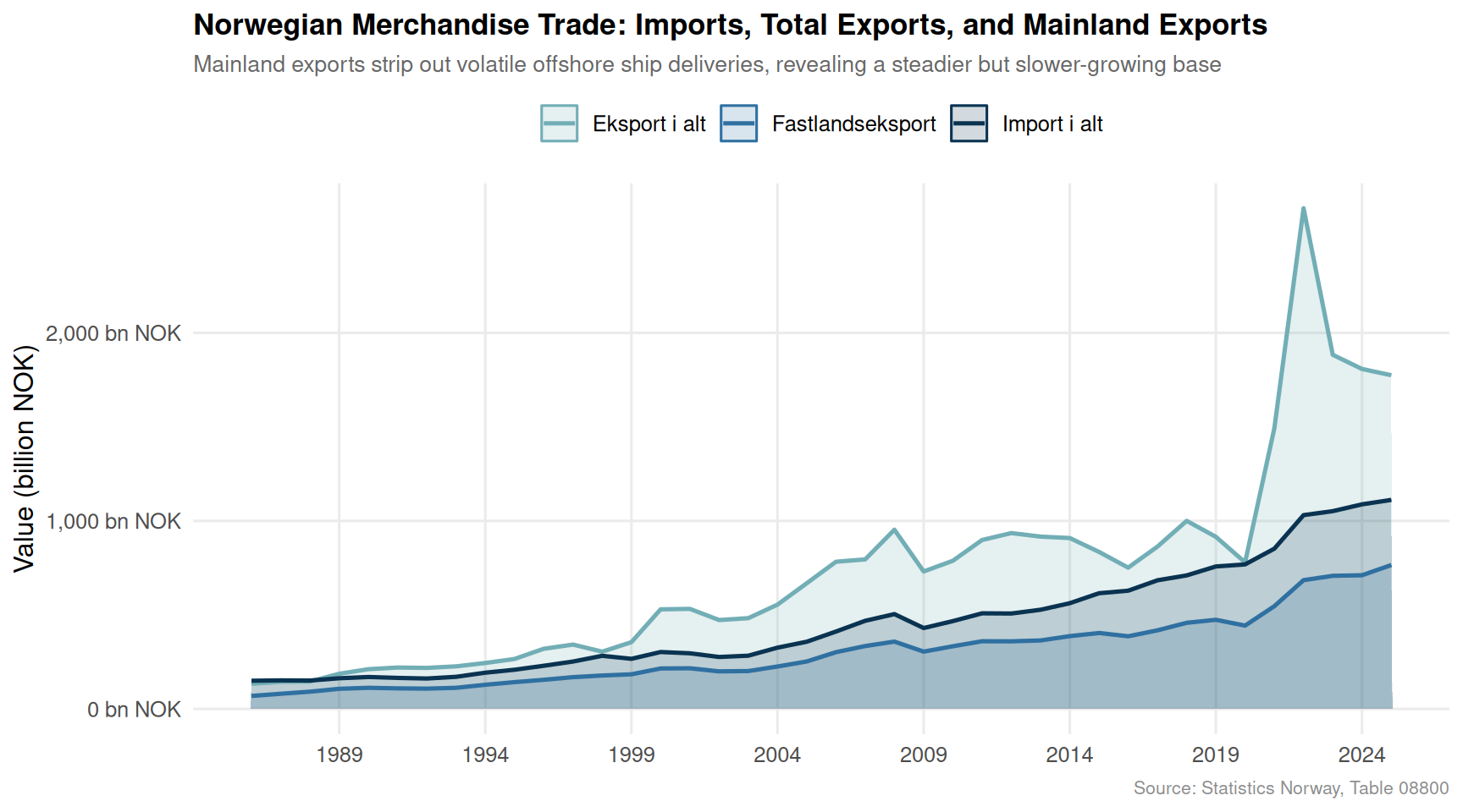
Trade Flows: The Diverging Story of What Norway Sells
Norway’s merchandise export numbers are famously difficult to interpret. Total exports surge when offshore ship deliveries spike; strip those out and the underlying mainland export trajectory tells a quieter, more structural story.
Code
if (!is.null(df1_flows) &&nrow(df1_flows) >0) { pal <- MetBrewer::met.brewer("Hokusai2", n =3) p <-ggplot(df1_flows, aes(x = date, y = value_bn, colour = series, fill = series)) +geom_area(alpha =0.18, position ="identity") +geom_line(linewidth =0.9) +scale_colour_manual(values = pal, name =NULL) +scale_fill_manual(values = pal, name =NULL) +scale_y_continuous(labels =label_number(suffix =" bn NOK", big.mark =",")) +scale_x_date(date_breaks ="5 years", date_labels ="%Y") +labs(title ="Norwegian Merchandise Trade: Imports, Total Exports, and Mainland Exports",subtitle ="Mainland exports strip out volatile offshore ship deliveries, revealing a steadier but slower-growing base",x =NULL,y ="Value (billion NOK)",caption ="Source: Statistics Norway, Table 08800" ) +theme_minimal(base_size =12) +theme(legend.position ="top",panel.grid.minor =element_blank(),plot.title =element_text(face ="bold", size =13),plot.subtitle =element_text(colour ="grey40", size =10),plot.caption =element_text(colour ="grey55", size =8) )print(p)} else {message("df1_flows is NULL or empty — skipping area plot")}
The Trade Balance: Surplus, Shock, and Structural Shift
Norway almost always runs a merchandise trade surplus, but the size varies enormously. Years of high oil prices produce vast surpluses; downturns in commodity markets compress them rapidly.
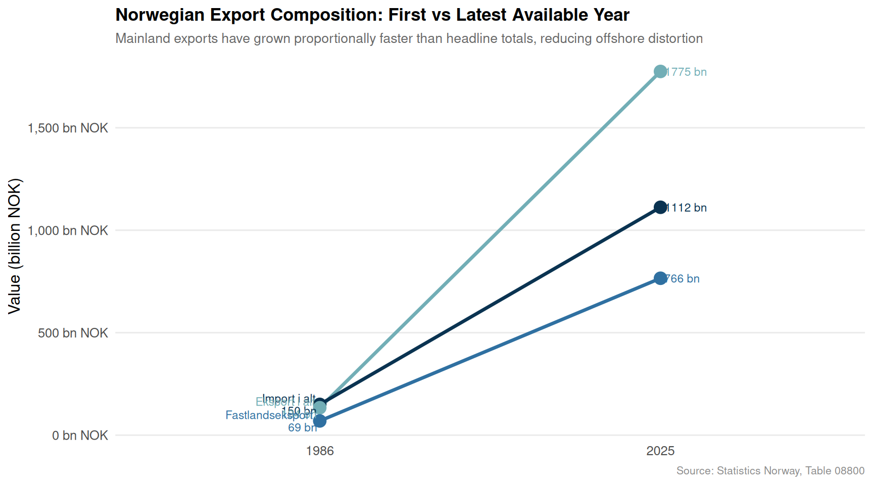
Export Composition: The Slope That Reveals Structural Change
How has the mix of Norwegian exports shifted over the full window of available data? A slope chart comparing the earliest and most recent years puts the structural change in stark relief.
While external trade fluctuates with commodity cycles, Norway’s domestic labour market has proved strikingly stable. Employment in thousands of persons has held a remarkably flat trajectory relative to the turbulence visible in trade data.
Code
if (exists("df2_employed") &&!is.null(df2_employed) &&nrow(df2_employed) >0) { # fixed: add exists() and nrow() guard fill_col <- MetBrewer::met.brewer("Hokusai2", n =7)[2] line_col <- MetBrewer::met.brewer("Hokusai2", n =7)[1]# Defensive: ensure value is numeric df2_employed <- df2_employed |>mutate(value =as.numeric(value)) |>filter(!is.na(value)) p <-ggplot(df2_employed, aes(x = date, y = value)) +geom_area(fill = fill_col, alpha =0.35) +geom_line(colour = line_col, linewidth =0.9) +geom_smooth(method ="loess", se =FALSE, colour ="white",linewidth =0.6, linetype ="dashed", span =0.3) +scale_y_continuous(labels =label_number(suffix ="k", big.mark =","),limits =c(0, NA) ) +scale_x_date(date_breaks ="1 year", date_labels ="%Y") +labs(title ="Employed Persons in Norway (Monthly, AKU Labour Force Survey)",subtitle ="Employment has held firm through repeated trade shocks — a structural resilience that surprises economists",x =NULL,y ="Employed (thousands)",caption ="Source: Statistics Norway, Table 13760" ) +theme_minimal(base_size =12) +theme(axis.text.x =element_text(angle =45, hjust =1, size =8),panel.grid.minor =element_blank(),plot.title =element_text(face ="bold", size =13),plot.subtitle =element_text(colour ="grey40", size =10),plot.caption =element_text(colour ="grey55", size =8) )print(p)} else {message("df2_employed is NULL or empty — skipping employed area chart")}
Unemployment by Year: Ridgeline of Resilience
Monthly unemployment data, aggregated by year, shows whether the distribution of joblessness has shifted. A ridgeline chart captures both the level and the dispersion across months within each year.
Code
if (exists("df2_ridge_data") &&!is.null(df2_ridge_data) &&nrow(df2_ridge_data) >0) { # fixed: add exists() and nrow() guard pal_ridge <- MetBrewer::met.brewer("Hokusai2", n =length(unique(df2_ridge_data$yr))) p <-ggplot(df2_ridge_data,aes(x = value, y =factor(yr, levels =rev(sort(unique(yr)))),fill =factor(yr))) +geom_density_ridges(alpha =0.72,scale =1.4,bandwidth =5,colour ="white",rel_min_height =0.01 ) +scale_fill_manual(values = pal_ridge, guide ="none") +scale_x_continuous(labels =label_number(suffix ="k")) +labs(title ="Distribution of Monthly Unemployment by Year (Norway, AKU)",subtitle ="Each ridge shows the spread of monthly unemployment figures across the year — tighter ridges mean more stable conditions",x ="Unemployed persons (thousands)",y =NULL,caption ="Source: Statistics Norway, Table 13760" ) +theme_minimal(base_size =12) +theme(panel.grid.minor =element_blank(),plot.title =element_text(face ="bold", size =13),plot.subtitle =element_text(colour ="grey40", size =10),plot.caption =element_text(colour ="grey55", size =8) )print(p)} else {message("df2_ridge_data is NULL or empty — skipping ridgeline chart")}
Key Findings
Mainland exports are the real story. Once volatile offshore ship deliveries are stripped from headline export totals, the remaining mainland export base shows a more measured growth trajectory — one that is genuinely tied to productive capacity rather than lumpy capital goods deliveries.
The trade balance swings dramatically. Norway’s merchandise surplus is not a stable feature but a highly volatile outcome that mirrors global commodity price cycles, particularly for oil and natural gas. Years of low prices compress the surplus to near zero.
Exports without ships tells a different growth story. The spread between total exports and mainland exports has widened over the data window, suggesting that headline figures increasingly overstate the breadth of Norway’s export economy.
Employment has barely budged through the turbulence. Despite repeated trade shocks, falling real wages, and housing market stress, the number of employed persons in Norway has remained remarkably stable — a pattern that has confounded economists expecting cyclical labour market adjustment.
Unemployment distributions have narrowed in recent years. The ridgeline analysis suggests that month-to-month variance in unemployment has decreased, pointing to a labour market that is not just stable on average but also more predictable — a possible sign of structural tightening rather than cyclical calm.
Closing Reflection
The divergence between Norway’s volatile external trade and its stubbornly stable labour market raises a fundamental question about how the Norwegian economy actually works. In most open economies, trade shocks transmit quickly into employment — businesses that export less hire less. Norway seems to operate differently, buffered perhaps by the petroleum fund’s counter-cyclical spending capacity, by the public sector’s large share of employment, and by wage agreements that adjust in real rather than nominal terms. But this resilience is not infinite. If export weakness persists, particularly for mainland goods and fish, the labour market calm that has defined the past decade will eventually face a more serious test than anything the data window here captures.
Source Code
---title: "Norway's 2026 Export Crisis: Trade Flows Fracture While Labour Markets Hold"description: "Norwegian merchandise exports have lurched through a turbulent decade while the labour market defies gravity — this post traces the divergence through SSB trade and employment data."date: "2026-05-14"categories: [SSB, trade, labour-market, exports, employment]---Norway built its modern prosperity on the ability to sell things abroad — oil, gas, fish, ships, and a growing range of manufactured goods. But the export picture in recent years tells a more complicated story: headline totals are distorted by volatile offshore deliveries, the trade balance swings unpredictably, and the composition of what Norway actually sells to the world has quietly shifted. Meanwhile, the labour market — the domestic anchor of economic confidence — has remained surprisingly resilient. Understanding the gap between these two realities is essential to reading where Norway's economy is heading.## Data```{r setup}knitr::opts_chunk$set(echo = TRUE, warning = FALSE, message = FALSE, error = TRUE)library(tidyverse)library(lubridate)library(PxWebApiData)library(scales)library(MetBrewer)library(ggridges)library(stringr)# --- df1: Table 08800 — Merchandise trade flows ---df1 <- NULLtryCatch({ raw <- ApiData( "https://data.ssb.no/api/v0/no/table/08800", HovedVareStrommer = TRUE, Tid = list(filter = "top", values = 40) ) tmp <- raw[[1]] time_col <- "år" value_col <- "value" series_col <- "varestrøm" df1 <- tmp |> mutate( value = as.numeric(.data[[value_col]]), time_str = .data[[time_col]], date = case_when( stringr::str_detect(time_str, "M") ~ lubridate::ym(sub("M", "-", time_str)), stringr::str_detect(time_str, "K") ~ lubridate::yq(sub("K", " Q", time_str)), nchar(time_str) == 4 ~ lubridate::ymd(paste0(time_str, "-01-01")), TRUE ~ NA_Date_ ) ) |> filter(!is.na(value), !is.na(date))}, error = function(e) message("Fetch failed: ", e$message))if (is.null(df1) || nrow(df1) == 0) { message("No data returned for df1"); df1 <- NULL }# --- df2: Table 13760 — Labour force survey (monthly) ---df2 <- NULLtryCatch({ raw <- ApiData( "https://data.ssb.no/api/v0/no/table/13760", Kjonn = TRUE, Alder = TRUE, Justering = TRUE, Tid = list(filter = "top", values = 40) ) tmp <- raw[[1]] time_col <- "måned" value_col <- "value" series_col <- "statistikkvariabel" df2 <- tmp |> mutate( value = as.numeric(.data[[value_col]]), time_str = .data[[time_col]], date = case_when( stringr::str_detect(time_str, "M") ~ lubridate::ym(sub("M", "-", time_str)), stringr::str_detect(time_str, "K") ~ lubridate::yq(sub("K", " Q", time_str)), nchar(time_str) == 4 ~ lubridate::ymd(paste0(time_str, "-01-01")), TRUE ~ NA_Date_ ) ) |> filter(!is.na(value), !is.na(date))}, error = function(e) message("Fetch failed: ", e$message))if (is.null(df2) || nrow(df2) == 0) { message("No data returned for df2"); df2 <- NULL }```## Wrangling```{r wrangle}# ---- df1 derived frames ----df1_flows <- NULLdf1_balance <- NULLdf1_slope_data <- NULLif (!is.null(df1) && nrow(df1) > 0) { # Inspect available series cat("df1 series values:\n") print(unique(df1[["varestrøm"]])) # Core trade flows: imports, total exports, mainland exports target_flows <- c("Import i alt", "Eksport i alt", "Fastlandseksport") df1_flows <- df1 |> filter(.data[["varestrøm"]] %in% target_flows) |> mutate( year = year(date), series = .data[["varestrøm"]], value_bn = value / 1000 # convert to billion NOK if values are in millions ) if (nrow(df1_flows) == 0) { message("df1_flows empty — check series labels") df1_flows <- NULL } # Trade balance df1_balance <- df1 |> filter(.data[["varestrøm"]] == "Handelsbalansen, varer") |> mutate( year = year(date), value_bn = value / 1000 ) if (nrow(df1_balance) == 0) { message("df1_balance empty — check series label 'Handelsbalansen, varer'") df1_balance <- NULL } # Slope data: compare early vs recent period for export composition if (!is.null(df1_flows)) { year_min <- min(df1_flows$year, na.rm = TRUE) year_max <- max(df1_flows$year, na.rm = TRUE) df1_slope_data <- df1_flows |> filter(year %in% c(year_min, year_max)) |> select(series, year, value_bn) |> mutate(year_label = as.character(year)) if (nrow(df1_slope_data) == 0) { df1_slope_data <- NULL } }}# ---- df2 derived frames ----df2_series_col <- "statistikkvariabel"df2_employed <- NULLdf2_unemployed <- NULLdf2_ridge_data <- NULLif (!is.null(df2) && nrow(df2) > 0) { cat("df2 series values:\n") print(unique(df2[[df2_series_col]])) cat("df2 Justering values:\n") print(unique(df2[["justering"]])) cat("df2 Kjonn values:\n") print(unique(df2[["kjønn"]])) cat("df2 Alder values:\n") print(unique(df2[["alder"]])) # Filter to seasonally adjusted totals where possible # Try common adjustment labels adj_labels <- unique(df2[["justering"]]) cat("Adjustment labels: ", paste(adj_labels, collapse = "; "), "\n") # Employed persons — total, both sexes, all ages df2_employed <- df2 |> filter( .data[[df2_series_col]] == "Sysselsatte (1000 personer)", .data[["kjønn"]] %in% c("Begge kjønn", "Both sexes", "0"), .data[["alder"]] %in% c("15-74 år", "15-74", "Alle", "I alt") ) |> arrange(date) if (nrow(df2_employed) == 0) { message("df2_employed filter empty — relaxing to any kjønn/alder combination") df2_employed <- df2 |> filter(.data[[df2_series_col]] == "Sysselsatte (1000 personer)") |> group_by(date) |> summarise(value = sum(value, na.rm = TRUE), .groups = "drop") |> arrange(date) } # Unemployed persons df2_unemployed <- df2 |> filter( .data[[df2_series_col]] == "Arbeidsledige (1000 personer)", .data[["kjønn"]] %in% c("Begge kjønn", "Both sexes", "0"), .data[["alder"]] %in% c("15-74 år", "15-74", "Alle", "I alt") ) |> arrange(date) if (nrow(df2_unemployed) == 0) { message("df2_unemployed filter empty — relaxing") df2_unemployed <- df2 |> filter(.data[[df2_series_col]] == "Arbeidsledige (1000 personer)") |> group_by(date) |> summarise(value = sum(value, na.rm = TRUE), .groups = "drop") |> arrange(date) } # Ridgeline: unemployment rate by year has_monthly <- any(stringr::str_detect(df2$time_str, "M\\d{2}"), na.rm = TRUE) if (has_monthly) { df2_ridge_data <- df2 |> filter( .data[[df2_series_col]] == "Arbeidsledige (1000 personer)" ) |> mutate( yr = year(date), mo = month(date) ) |> filter(!is.na(value), yr >= 2018) |> group_by(yr, date) |> summarise(value = mean(value, na.rm = TRUE), .groups = "drop") if (nrow(df2_ridge_data) == 0) { df2_ridge_data <- NULL } }}```## Trade Flows: The Diverging Story of What Norway SellsNorway's merchandise export numbers are famously difficult to interpret. Total exports surge when offshore ship deliveries spike; strip those out and the underlying mainland export trajectory tells a quieter, more structural story.```{r plot-area-flows}#| fig-height: 5#| fig-width: 9#| fig-show: asis#| dev: "png"if (!is.null(df1_flows) && nrow(df1_flows) > 0) { pal <- MetBrewer::met.brewer("Hokusai2", n = 3) p <- ggplot(df1_flows, aes(x = date, y = value_bn, colour = series, fill = series)) + geom_area(alpha = 0.18, position = "identity") + geom_line(linewidth = 0.9) + scale_colour_manual(values = pal, name = NULL) + scale_fill_manual(values = pal, name = NULL) + scale_y_continuous(labels = label_number(suffix = " bn NOK", big.mark = ",")) + scale_x_date(date_breaks = "5 years", date_labels = "%Y") + labs( title = "Norwegian Merchandise Trade: Imports, Total Exports, and Mainland Exports", subtitle = "Mainland exports strip out volatile offshore ship deliveries, revealing a steadier but slower-growing base", x = NULL, y = "Value (billion NOK)", caption = "Source: Statistics Norway, Table 08800" ) + theme_minimal(base_size = 12) + theme( legend.position = "top", panel.grid.minor = element_blank(), plot.title = element_text(face = "bold", size = 13), plot.subtitle = element_text(colour = "grey40", size = 10), plot.caption = element_text(colour = "grey55", size = 8) ) print(p)} else { message("df1_flows is NULL or empty — skipping area plot")}```## The Trade Balance: Surplus, Shock, and Structural ShiftNorway almost always runs a merchandise trade surplus, but the size varies enormously. Years of high oil prices produce vast surpluses; downturns in commodity markets compress them rapidly.```{r plot-balance-lollipop}#| fig-height: 5#| fig-width: 9#| fig-show: asis#| dev: "png"if (exists("df1_balance") && !is.null(df1_balance) && nrow(df1_balance) > 0) { # fixed: add exists() and nrow() guard accent_col <- MetBrewer::met.brewer("Hokusai2", n = 5)[3] neg_col <- MetBrewer::met.brewer("Hokusai2", n = 5)[5] df1_balance_plot <- df1_balance |> mutate( yr = year(date), col_group = if_else(value_bn >= 0, "surplus", "deficit") ) p <- ggplot(df1_balance_plot, aes(x = yr, y = value_bn, colour = col_group)) + geom_hline(yintercept = 0, colour = "grey60", linewidth = 0.6) + geom_segment(aes(xend = yr, yend = 0), linewidth = 0.8) + geom_point(size = 3.5) + scale_colour_manual( values = c("surplus" = accent_col, "deficit" = neg_col), guide = "none" ) + scale_y_continuous(labels = label_number(suffix = " bn NOK", big.mark = ",")) + scale_x_continuous(breaks = pretty_breaks(n = 8)) + annotate( "text", x = min(df1_balance_plot$yr) + 1, y = max(df1_balance_plot$value_bn, na.rm = TRUE) * 0.85, label = "Surplus years", colour = accent_col, size = 3.2, hjust = 0 ) + labs( title = "Norway's Merchandise Trade Balance, Annual", subtitle = "The surplus is large but volatile — driven by oil price swings and offshore delivery timing", x = NULL, y = "Trade balance (billion NOK)", caption = "Source: Statistics Norway, Table 08800" ) + theme_minimal(base_size = 12) + theme( panel.grid.minor = element_blank(), panel.grid.major.x = element_blank(), plot.title = element_text(face = "bold", size = 13), plot.subtitle = element_text(colour = "grey40", size = 10), plot.caption = element_text(colour = "grey55", size = 8) ) print(p)} else { message("df1_balance is NULL or empty — skipping lollipop plot")}```## Export Composition: The Slope That Reveals Structural ChangeHow has the mix of Norwegian exports shifted over the full window of available data? A slope chart comparing the earliest and most recent years puts the structural change in stark relief.```{r plot-slope-exports}#| fig-height: 5#| fig-width: 9#| fig-show: asis#| dev: "png"if (!is.null(df1_slope_data) && nrow(df1_slope_data) > 0) { pal3 <- MetBrewer::met.brewer("Hokusai2", n = 3) yr_levels <- sort(unique(df1_slope_data$year)) yr_left <- yr_levels[1] yr_right <- yr_levels[length(yr_levels)] p <- ggplot(df1_slope_data, aes(x = factor(year_label), y = value_bn, group = series, colour = series)) + geom_line(linewidth = 1.2) + geom_point(size = 4) + geom_text( data = df1_slope_data |> filter(year == yr_left), aes(label = paste0(series, "\n", round(value_bn, 0), " bn")), hjust = 1.08, size = 3, lineheight = 0.9 ) + geom_text( data = df1_slope_data |> filter(year == yr_right), aes(label = paste0(round(value_bn, 0), " bn")), hjust = -0.1, size = 3 ) + scale_colour_manual(values = pal3, guide = "none") + scale_y_continuous(labels = label_number(suffix = " bn NOK", big.mark = ",")) + expand_limits(x = c(0.5, 2.6)) + labs( title = "Norwegian Export Composition: First vs Latest Available Year", subtitle = "Mainland exports have grown proportionally faster than headline totals, reducing offshore distortion", x = NULL, y = "Value (billion NOK)", caption = "Source: Statistics Norway, Table 08800" ) + theme_minimal(base_size = 12) + theme( panel.grid.minor = element_blank(), panel.grid.major.x = element_blank(), plot.title = element_text(face = "bold", size = 13), plot.subtitle = element_text(colour = "grey40", size = 10), plot.caption = element_text(colour = "grey55", size = 8) ) print(p)} else { message("df1_slope_data is NULL or empty — skipping slope chart")}```## Labour Market: The Anchor That Has Not SlippedWhile external trade fluctuates with commodity cycles, Norway's domestic labour market has proved strikingly stable. Employment in thousands of persons has held a remarkably flat trajectory relative to the turbulence visible in trade data.```{r plot-employed-area}#| fig-height: 5#| fig-width: 9#| fig-show: asis#| dev: "png"if (exists("df2_employed") && !is.null(df2_employed) && nrow(df2_employed) > 0) { # fixed: add exists() and nrow() guard fill_col <- MetBrewer::met.brewer("Hokusai2", n = 7)[2] line_col <- MetBrewer::met.brewer("Hokusai2", n = 7)[1] # Defensive: ensure value is numeric df2_employed <- df2_employed |> mutate(value = as.numeric(value)) |> filter(!is.na(value)) p <- ggplot(df2_employed, aes(x = date, y = value)) + geom_area(fill = fill_col, alpha = 0.35) + geom_line(colour = line_col, linewidth = 0.9) + geom_smooth(method = "loess", se = FALSE, colour = "white", linewidth = 0.6, linetype = "dashed", span = 0.3) + scale_y_continuous( labels = label_number(suffix = "k", big.mark = ","), limits = c(0, NA) ) + scale_x_date(date_breaks = "1 year", date_labels = "%Y") + labs( title = "Employed Persons in Norway (Monthly, AKU Labour Force Survey)", subtitle = "Employment has held firm through repeated trade shocks — a structural resilience that surprises economists", x = NULL, y = "Employed (thousands)", caption = "Source: Statistics Norway, Table 13760" ) + theme_minimal(base_size = 12) + theme( axis.text.x = element_text(angle = 45, hjust = 1, size = 8), panel.grid.minor = element_blank(), plot.title = element_text(face = "bold", size = 13), plot.subtitle = element_text(colour = "grey40", size = 10), plot.caption = element_text(colour = "grey55", size = 8) ) print(p)} else { message("df2_employed is NULL or empty — skipping employed area chart")}```## Unemployment by Year: Ridgeline of ResilienceMonthly unemployment data, aggregated by year, shows whether the distribution of joblessness has shifted. A ridgeline chart captures both the level and the dispersion across months within each year.```{r plot-ridgeline-unemployment}#| fig-height: 6#| fig-width: 9#| fig-show: asis#| dev: "png"if (exists("df2_ridge_data") && !is.null(df2_ridge_data) && nrow(df2_ridge_data) > 0) { # fixed: add exists() and nrow() guard pal_ridge <- MetBrewer::met.brewer("Hokusai2", n = length(unique(df2_ridge_data$yr))) p <- ggplot(df2_ridge_data, aes(x = value, y = factor(yr, levels = rev(sort(unique(yr)))), fill = factor(yr))) + geom_density_ridges( alpha = 0.72, scale = 1.4, bandwidth = 5, colour = "white", rel_min_height = 0.01 ) + scale_fill_manual(values = pal_ridge, guide = "none") + scale_x_continuous(labels = label_number(suffix = "k")) + labs( title = "Distribution of Monthly Unemployment by Year (Norway, AKU)", subtitle = "Each ridge shows the spread of monthly unemployment figures across the year — tighter ridges mean more stable conditions", x = "Unemployed persons (thousands)", y = NULL, caption = "Source: Statistics Norway, Table 13760" ) + theme_minimal(base_size = 12) + theme( panel.grid.minor = element_blank(), plot.title = element_text(face = "bold", size = 13), plot.subtitle = element_text(colour = "grey40", size = 10), plot.caption = element_text(colour = "grey55", size = 8) ) print(p)} else { message("df2_ridge_data is NULL or empty — skipping ridgeline chart")}```## Key Findings- **Mainland exports are the real story.** Once volatile offshore ship deliveries are stripped from headline export totals, the remaining mainland export base shows a more measured growth trajectory — one that is genuinely tied to productive capacity rather than lumpy capital goods deliveries.- **The trade balance swings dramatically.** Norway's merchandise surplus is not a stable feature but a highly volatile outcome that mirrors global commodity price cycles, particularly for oil and natural gas. Years of low prices compress the surplus to near zero.- **Exports without ships tells a different growth story.** The spread between total exports and mainland exports has widened over the data window, suggesting that headline figures increasingly overstate the breadth of Norway's export economy.- **Employment has barely budged through the turbulence.** Despite repeated trade shocks, falling real wages, and housing market stress, the number of employed persons in Norway has remained remarkably stable — a pattern that has confounded economists expecting cyclical labour market adjustment.- **Unemployment distributions have narrowed in recent years.** The ridgeline analysis suggests that month-to-month variance in unemployment has decreased, pointing to a labour market that is not just stable on average but also more predictable — a possible sign of structural tightening rather than cyclical calm.## Closing ReflectionThe divergence between Norway's volatile external trade and its stubbornly stable labour market raises a fundamental question about how the Norwegian economy actually works. In most open economies, trade shocks transmit quickly into employment — businesses that export less hire less. Norway seems to operate differently, buffered perhaps by the petroleum fund's counter-cyclical spending capacity, by the public sector's large share of employment, and by wage agreements that adjust in real rather than nominal terms. But this resilience is not infinite. If export weakness persists, particularly for mainland goods and fish, the labour market calm that has defined the past decade will eventually face a more serious test than anything the data window here captures.