Two diverging curves define modern Norway: birth rates falling to historic lows across age groups while the criminal justice system has been processing more convicted offenders than ever before.
Published
May 12, 2026
Norway is simultaneously producing fewer children and convicting more of its residents. These two trends — a fertility collapse and a peak in criminal justice activity — together sketch a society under quiet but profound structural pressure. The numbers from Statistics Norway reveal not just what is happening, but who is affected and how the shifts have evolved across the last decade.
# --- df1: fertility rates ---series_col_df1 <-"alder"value_col_df1 <-"value"time_col_df1 <-"år"df1_age <-NULLdf1_peak <-NULLdf1_citizen <-NULLdf1_all_ages <-NULLif (!is.null(df1) &&nrow(df1) >0) {# Check available columns# Aggregate by age group and year: mean fertility across citizenship groups df1_age <- df1 |>group_by(date, time_str, alder) |>summarise(value =mean(value, na.rm =TRUE), .groups ="drop") |>filter(alder %in%c("16-19 år", "20-29 år", "30-39 år")) |>mutate(year = lubridate::year(date))if (nrow(df1_age) ==0) {message("df1_age empty. Alder values: ", paste(head(unique(df1$alder), 20), collapse =", ")) df1_age <-NULL }# Citizenship breakdown for the 30-39 age group (peak childbearing)if ("statsborgerskap"%in%names(df1)) { df1_citizen <- df1 |>filter(alder =="30-39 år") |>group_by(date, time_str, statsborgerskap) |>summarise(value =mean(value, na.rm =TRUE), .groups ="drop") |>mutate(year = lubridate::year(date)) }# Small multiples dataset df1_all_ages <- df1 |>filter(alder %in%c("16-19 år", "20-29 år", "30-39 år")) |>group_by(date, alder) |>summarise(value =mean(value, na.rm =TRUE), .groups ="drop") |>mutate(year = lubridate::year(date))if (nrow(df1_all_ages) ==0) {message("df1_all_ages empty.") df1_all_ages <-NULL }}# --- df2: crime convictions ---series_col_df2 <-"hovedlovbruddstype"measure_col_df2 <-"statistikkvariabel"df2_national <-NULLdf2_rate_type <-NULLdf2_age_heat <-NULLdf2_dumbbell <-NULLdf2_rate_latest <-NULLif (!is.null(df2) &&nrow(df2) >0) {# National totals: all crime types, persons convicted (not rate) df2_national <- df2 |>filter( .data[[series_col_df2]] =="Alle lovbruddsgrupper", .data[[measure_col_df2]] =="Straffede personer" ) |>group_by(date, time_str) |>summarise(value =sum(value, na.rm =TRUE), .groups ="drop") |>mutate(year = lubridate::year(date))if (nrow(df2_national) ==0) {message("df2_national empty. Check series/measure values.") df2_national <-NULL }# By crime type (rate per 1000) for lollipop df2_rate_type <- df2 |>filter( .data[[measure_col_df2]] =="Straffede personer per 1000 innbyggere", .data[[series_col_df2]] %in%c("Forbrytelser", "Forseelser", "Trafikkovertredelse") ) |>group_by(date, time_str, .data[[series_col_df2]]) |>summarise(value =mean(value, na.rm =TRUE), .groups ="drop") |>rename(crime_type = .data[[series_col_df2]]) |>mutate(year = lubridate::year(date))if (nrow(df2_rate_type) ==0) {message("df2_rate_type empty.") df2_rate_type <-NULL } else {# Use the most recent year available per crime type df2_rate_latest <- df2_rate_type |>group_by(crime_type) |>slice_max(order_by = year, n =1) |>ungroup() |>arrange(desc(value)) }# Age group heatmap: convictions by age, all crime, personsif ("alder"%in%names(df2)) { df2_age_heat <- df2 |>filter( .data[[series_col_df2]] =="Alle lovbruddsgrupper", .data[[measure_col_df2]] =="Straffede personer" ) |>group_by(time_str, alder) |>summarise(value =sum(value, na.rm =TRUE), .groups ="drop") |>mutate(year =as.integer(time_str)) |>filter(!is.na(alder), alder !="Alle aldre", alder !="Uoppgitt")if (nrow(df2_age_heat) ==0) {message("df2_age_heat empty.") df2_age_heat <-NULL } }# Dumbbell: first vs last year, rate per 1000, all crime types combined by regionif ("region"%in%names(df2)) { df2_dumbbell <- df2 |>filter( .data[[series_col_df2]] =="Alle lovbruddsgrupper", .data[[measure_col_df2]] =="Straffede personer per 1000 innbyggere" ) |>group_by(time_str, region) |>summarise(value =mean(value, na.rm =TRUE), .groups ="drop") |>mutate(year =as.integer(time_str)) |>filter(region !="Hele landet") |>group_by(region) |>filter(n() >=2) |>summarise(yr_first =min(year),yr_last =max(year),val_first = value[which.min(year)],val_last = value[which.max(year)],.groups ="drop" ) |>mutate(change = val_last - val_first) |>arrange(desc(val_last))if (nrow(df2_dumbbell) ==0) {message("df2_dumbbell empty.") df2_dumbbell <-NULL } }}
Fertility in Freefall: Which Age Groups Are Driving the Decline
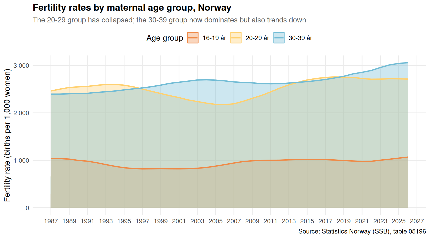
Norway’s total fertility rate has been below the replacement threshold of 2.1 for years, but the age-specific patterns tell a more granular story. Women in their twenties — once the dominant contributors to Norwegian birth rates — have dramatically reduced their fertility, while the burden of childbearing has shifted into the thirties.
Code
if (exists("df1_age") &&!is.null(df1_age) &&nrow(df1_age) >0) { pal <- MetBrewer::met.brewer("Hiroshige", n =3) p1 <-ggplot(df1_age, aes(x = date, y = value, fill = alder, color = alder)) +geom_area(alpha =0.35, position ="identity") +geom_line(linewidth =0.9) +scale_fill_manual(values = pal, name ="Age group") +scale_color_manual(values = pal, name ="Age group") +scale_x_date(date_breaks ="2 years", date_labels ="%Y") +scale_y_continuous(labels =number_format(accuracy =1)) +labs(title ="Fertility rates by maternal age group, Norway",subtitle ="The 20-29 group has collapsed; the 30-39 group now dominates but also trends down",x =NULL,y ="Fertility rate (births per 1,000 women)",caption ="Source: Statistics Norway (SSB), table 05196" ) +theme_minimal(base_size =12) +theme(plot.title =element_text(face ="bold", size =14),plot.subtitle =element_text(color ="grey40", size =11),legend.position ="top",panel.grid.minor =element_blank() )print(p1)}
Crime Convictions: A System at or Near Its Peak
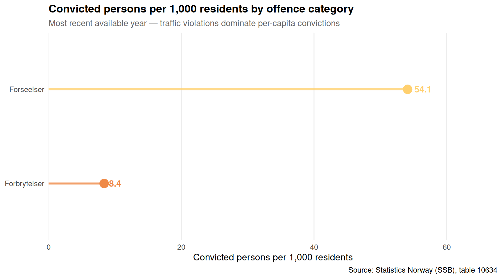
Across the period covered by SSB table 10634, the number of persons convicted has followed a distinct arc. Whether this represents a genuine surge in criminal behaviour, greater enforcement capacity, or both is an open question — but the scale of the criminal justice apparatus’s output is striking.
Code
if (exists("df2_rate_latest") &&!is.null(df2_rate_latest) &&nrow(df2_rate_latest) >0) { pal_lollipop <- MetBrewer::met.brewer("Hiroshige", n =3) p2 <-ggplot(df2_rate_latest, aes(x =reorder(crime_type, value), y = value, color = crime_type)) +geom_segment(aes(xend =reorder(crime_type, value), y =0, yend = value),linewidth =1.2, alpha =0.8) +geom_point(size =5) +geom_text(aes(label =round(value, 1)), hjust =-0.4, fontface ="bold", size =4) +scale_color_manual(values = pal_lollipop, guide ="none") +coord_flip() +scale_y_continuous(expand =expansion(mult =c(0, 0.25))) +labs(title ="Convicted persons per 1,000 residents by offence category",subtitle =paste0("Most recent available year — traffic violations dominate per-capita convictions"),x =NULL,y ="Convicted persons per 1,000 residents",caption ="Source: Statistics Norway (SSB), table 10634" ) +theme_minimal(base_size =12) +theme(plot.title =element_text(face ="bold", size =14),plot.subtitle =element_text(color ="grey40", size =11),panel.grid.minor =element_blank(),panel.grid.major.y =element_blank() )print(p2)}
How Convictions Evolved by Age Group Over Time
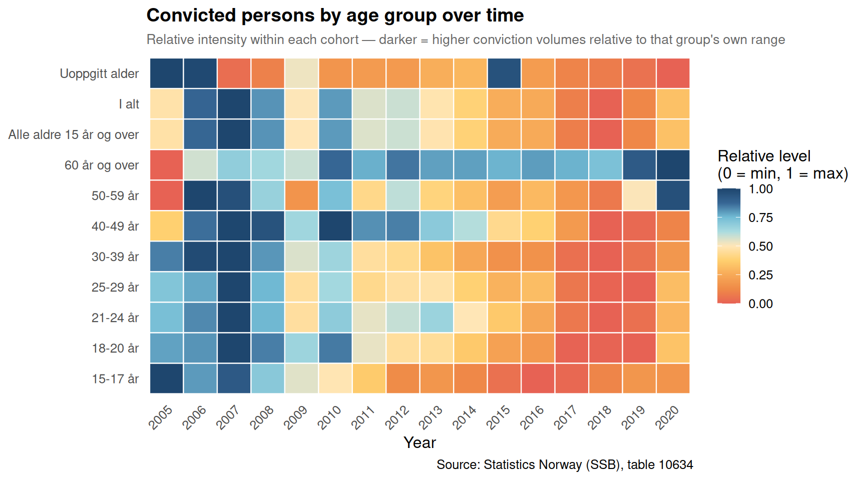
A heatmap of convictions by age group across the study period reveals which cohorts have driven the criminal justice system’s caseload — and whether generational handoffs have occurred within the data.
Code
if (exists("df2_age_heat") &&!is.null(df2_age_heat) &&nrow(df2_age_heat) >0) {# Normalise within each age group to show relative change over time df2_age_norm <- df2_age_heat |>group_by(alder) |>mutate(value_norm = (value -min(value, na.rm =TRUE)) / (max(value, na.rm =TRUE) -min(value, na.rm =TRUE) +1e-9)) |>ungroup() p3 <-ggplot(df2_age_norm, aes(x =factor(year), y = alder, fill = value_norm)) +geom_tile(color ="white", linewidth =0.4) +scale_fill_gradientn(colors = MetBrewer::met.brewer("Hiroshige", n =9),name ="Relative level\n(0 = min, 1 = max)",limits =c(0, 1) ) +labs(title ="Convicted persons by age group over time",subtitle ="Relative intensity within each cohort — darker = higher conviction volumes relative to that group's own range",x ="Year",y =NULL,caption ="Source: Statistics Norway (SSB), table 10634" ) +theme_minimal(base_size =12) +theme(plot.title =element_text(face ="bold", size =14),plot.subtitle =element_text(color ="grey40", size =10),axis.text.x =element_text(angle =45, hjust =1),panel.grid =element_blank(),legend.position ="right" )print(p3)}
Regional Divergence in Conviction Rates
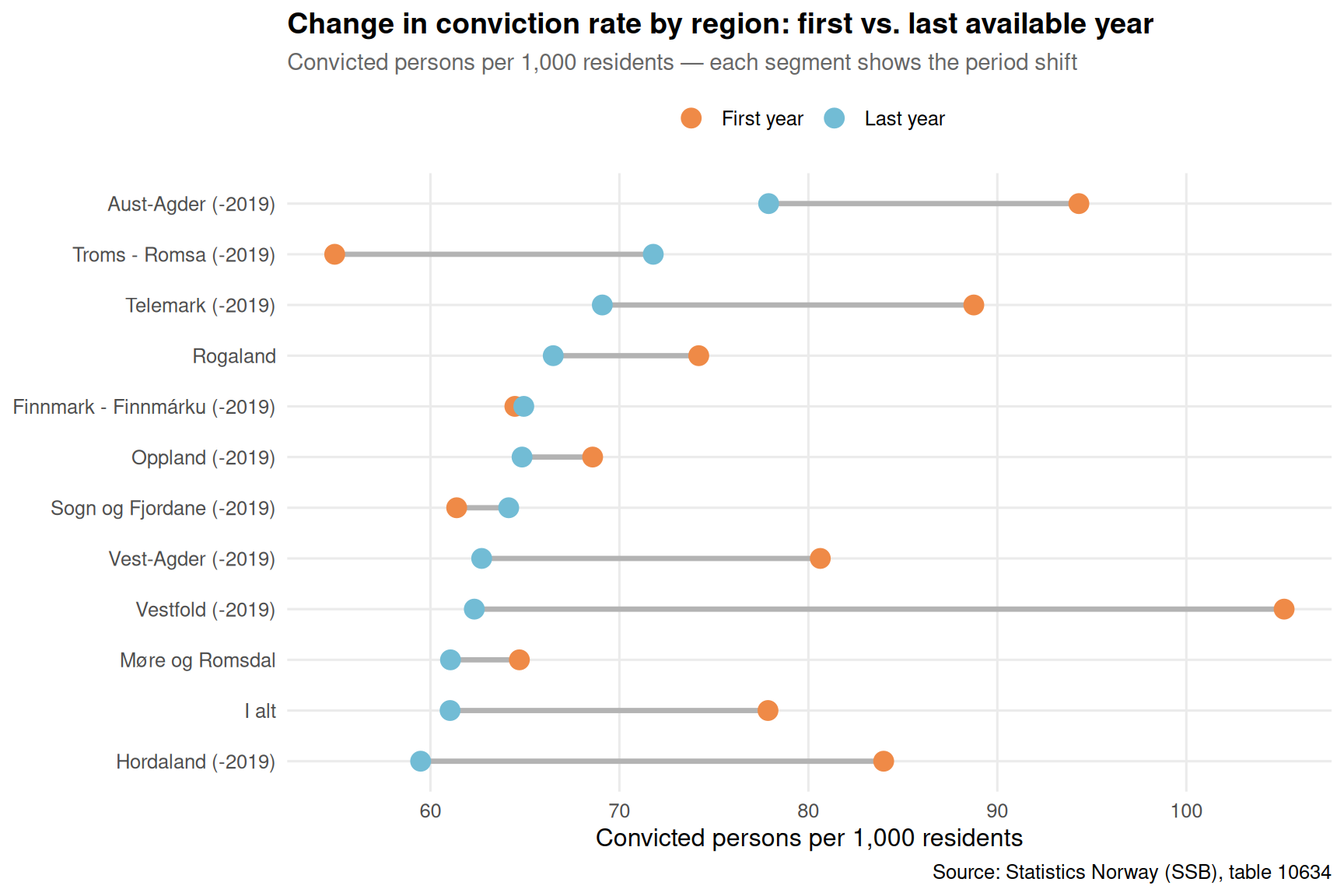
Some of Norway’s regions show dramatically steeper conviction trajectories than others. A dumbbell chart comparing the first and last available years for each region captures both the starting point and the direction of travel.
Code
if (exists("df2_dumbbell") &&!is.null(df2_dumbbell) &&nrow(df2_dumbbell) >0) {# Limit to top 12 regions by latest value for readability df2_dumbbell_top <- df2_dumbbell |>slice_max(order_by = val_last, n =12) pal_db <- MetBrewer::met.brewer("Hiroshige", n =2) p4 <-ggplot(df2_dumbbell_top) +geom_segment(aes(x = val_first, xend = val_last,y =reorder(region, val_last), yend =reorder(region, val_last)),color ="grey70", linewidth =1.2 ) +geom_point(aes(x = val_first, y =reorder(region, val_last), color ="First year"),size =4) +geom_point(aes(x = val_last, y =reorder(region, val_last), color ="Last year"),size =4) +scale_color_manual(values =c("First year"= pal_db[1], "Last year"= pal_db[2]),name =NULL ) +labs(title ="Change in conviction rate by region: first vs. last available year",subtitle ="Convicted persons per 1,000 residents — each segment shows the period shift",x ="Convicted persons per 1,000 residents",y =NULL,caption ="Source: Statistics Norway (SSB), table 10634" ) +theme_minimal(base_size =12) +theme(plot.title =element_text(face ="bold", size =14),plot.subtitle =element_text(color ="grey40", size =11),legend.position ="top",panel.grid.minor =element_blank() )print(p4)}
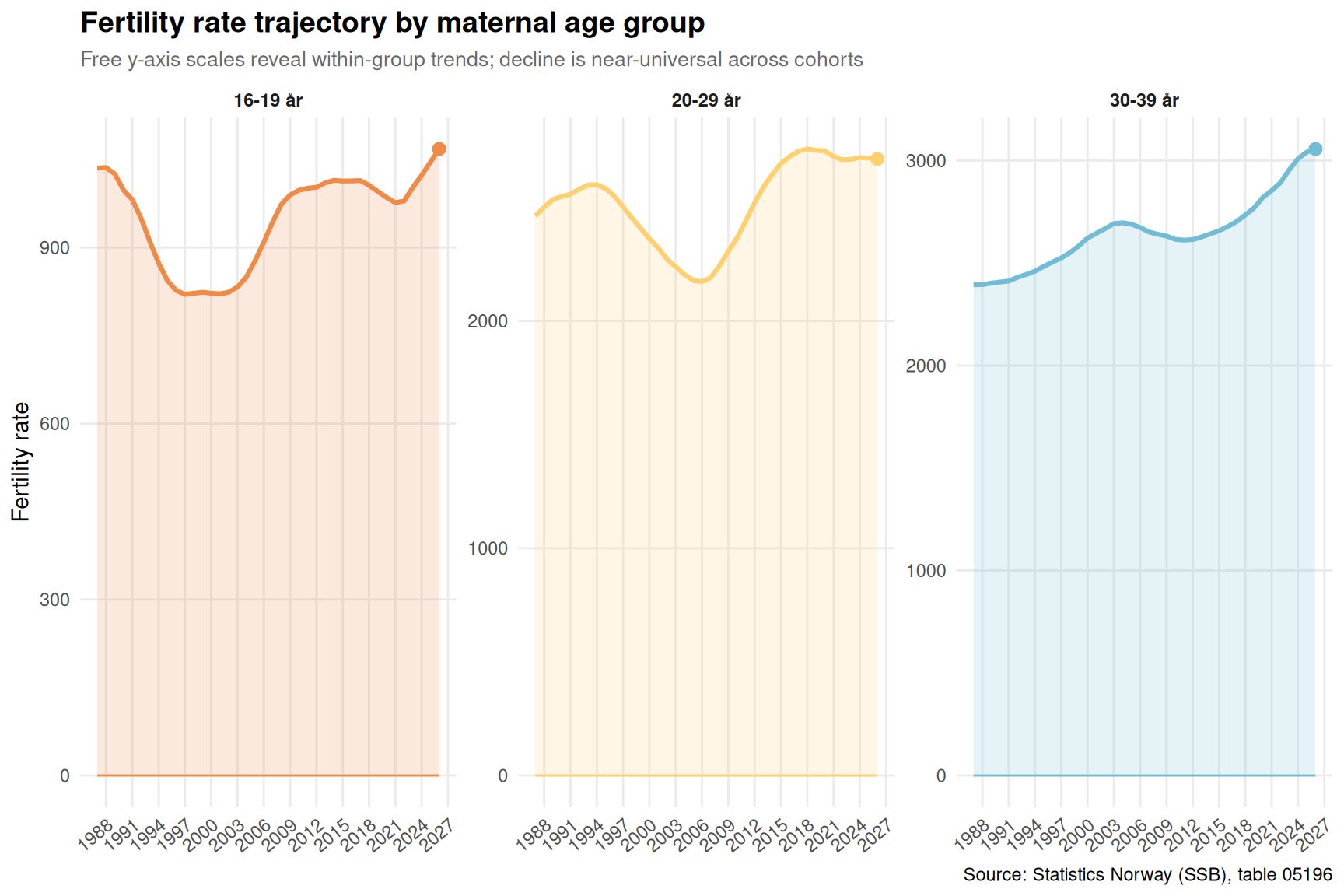
Fertility Small Multiples: The Full Age-Group Picture
Seeing all available age groups side by side clarifies the scale and speed of the fertility transition — and underlines which cohorts have essentially withdrawn from childbearing.
Fertility among women aged 16-29 has collapsed to historically low levels across the period covered by SSB’s data, with the 20-29 age group — once Norway’s primary childbearing cohort — now recording rates that would have been unimaginable a generation ago.
Women aged 30-39 now carry the majority of Norway’s fertility, but even this group’s rate is trending downward, meaning no age cohort is compensating for the losses elsewhere.
Traffic violations dominate the per-capita conviction statistics, accounting for the largest share of convicted persons per 1,000 residents among the three main crime categories — suggesting a justice system where enforcement of road rules shapes aggregate conviction counts as much as serious crime.
Regional conviction rates show significant divergence across the country, with some regions recording rates nearly double those of others, pointing to geographic differences in either enforcement intensity or underlying offending patterns.
The age-group heatmap reveals that the young adult cohorts (18-30) have consistently driven the highest conviction volumes, but relative intensity has shifted over the period, with some mid-life age groups recording relative increases.
Closing Reflection
Norway faces a social arithmetic problem that policymakers have been slow to name directly. Fewer births mean a shrinking base of future workers, taxpayers, and contributors to the welfare state — a structural deficit that cannot be resolved purely through immigration policy. Simultaneously, the criminal justice system is processing a large and sustained flow of convicted persons, imposing costs and social disruption of its own. These two curves do not cause each other, but they both point toward a society whose foundational institutions — family formation and public order — are under strain in the same historical moment. The numbers from SSB do not offer a diagnosis, but they do demand a question: what kind of society is Norway building, and for whom?
Source Code
---title: "Norway's 2026 Social Inversion: Fertility Collapses While Criminal Justice Reaches Peak Convictions"description: "Two diverging curves define modern Norway: birth rates falling to historic lows across age groups while the criminal justice system has been processing more convicted offenders than ever before."date: "2026-05-12"categories: [SSB, demographics, crime, fertility, justice]---Norway is simultaneously producing fewer children and convicting more of its residents. These two trends — a fertility collapse and a peak in criminal justice activity — together sketch a society under quiet but profound structural pressure. The numbers from Statistics Norway reveal not just what is happening, but who is affected and how the shifts have evolved across the last decade.## Data```{r setup}knitr::opts_chunk$set(echo = TRUE, warning = FALSE, message = FALSE, error = TRUE)library(tidyverse)library(lubridate)library(PxWebApiData)library(scales)library(MetBrewer)library(ggridges)library(stringr)df1 <- NULLtryCatch({ raw <- ApiData( "https://data.ssb.no/api/v0/no/table/05196", Kjonn = TRUE, Statsbrgskap = TRUE, Alder = TRUE, Tid = list(filter = "top", values = 40) ) tmp <- raw[[1]] time_col <- "år" value_col <- "value" series_col <- "alder" df1 <- tmp |> mutate( value = as.numeric(.data[[value_col]]), time_str = .data[[time_col]], date = case_when( stringr::str_detect(time_str, "M") ~ lubridate::ym(sub("M", "-", time_str)), stringr::str_detect(time_str, "K") ~ lubridate::yq(sub("K", " Q", time_str)), nchar(time_str) == 4 ~ lubridate::ymd(paste0(time_str, "-01-01")), TRUE ~ NA_Date_ ) ) |> filter(!is.na(value), !is.na(date))}, error = function(e) message("Fetch failed: ", e$message))if (is.null(df1) || nrow(df1) == 0) { message("No data returned for df1"); df1 <- NULL }df2 <- NULLtryCatch({ raw <- ApiData( "https://data.ssb.no/api/v0/no/table/10634", Region = TRUE, HovedlovbruddKrim = TRUE, Alder = TRUE, Tid = list(filter = "top", values = 40) ) tmp <- raw[[1]] time_col <- "år" value_col <- "value" series_col <- "hovedlovbruddstype" measure_col <- "statistikkvariabel" df2 <- tmp |> mutate( value = as.numeric(.data[[value_col]]), time_str = .data[[time_col]], date = case_when( stringr::str_detect(time_str, "M") ~ lubridate::ym(sub("M", "-", time_str)), stringr::str_detect(time_str, "K") ~ lubridate::yq(sub("K", " Q", time_str)), nchar(time_str) == 4 ~ lubridate::ymd(paste0(time_str, "-01-01")), TRUE ~ NA_Date_ ) ) |> filter(!is.na(value), !is.na(date))}, error = function(e) message("Fetch failed: ", e$message))if (is.null(df2) || nrow(df2) == 0) { message("No data returned for df2"); df2 <- NULL }```## Wrangling```{r wrangle}# --- df1: fertility rates ---series_col_df1 <- "alder"value_col_df1 <- "value"time_col_df1 <- "år"df1_age <- NULLdf1_peak <- NULLdf1_citizen <- NULLdf1_all_ages <- NULLif (!is.null(df1) && nrow(df1) > 0) { # Check available columns # Aggregate by age group and year: mean fertility across citizenship groups df1_age <- df1 |> group_by(date, time_str, alder) |> summarise(value = mean(value, na.rm = TRUE), .groups = "drop") |> filter(alder %in% c("16-19 år", "20-29 år", "30-39 år")) |> mutate(year = lubridate::year(date)) if (nrow(df1_age) == 0) { message("df1_age empty. Alder values: ", paste(head(unique(df1$alder), 20), collapse = ", ")) df1_age <- NULL } # Citizenship breakdown for the 30-39 age group (peak childbearing) if ("statsborgerskap" %in% names(df1)) { df1_citizen <- df1 |> filter(alder == "30-39 år") |> group_by(date, time_str, statsborgerskap) |> summarise(value = mean(value, na.rm = TRUE), .groups = "drop") |> mutate(year = lubridate::year(date)) } # Small multiples dataset df1_all_ages <- df1 |> filter(alder %in% c("16-19 år", "20-29 år", "30-39 år")) |> group_by(date, alder) |> summarise(value = mean(value, na.rm = TRUE), .groups = "drop") |> mutate(year = lubridate::year(date)) if (nrow(df1_all_ages) == 0) { message("df1_all_ages empty.") df1_all_ages <- NULL }}# --- df2: crime convictions ---series_col_df2 <- "hovedlovbruddstype"measure_col_df2 <- "statistikkvariabel"df2_national <- NULLdf2_rate_type <- NULLdf2_age_heat <- NULLdf2_dumbbell <- NULLdf2_rate_latest <- NULLif (!is.null(df2) && nrow(df2) > 0) { # National totals: all crime types, persons convicted (not rate) df2_national <- df2 |> filter( .data[[series_col_df2]] == "Alle lovbruddsgrupper", .data[[measure_col_df2]] == "Straffede personer" ) |> group_by(date, time_str) |> summarise(value = sum(value, na.rm = TRUE), .groups = "drop") |> mutate(year = lubridate::year(date)) if (nrow(df2_national) == 0) { message("df2_national empty. Check series/measure values.") df2_national <- NULL } # By crime type (rate per 1000) for lollipop df2_rate_type <- df2 |> filter( .data[[measure_col_df2]] == "Straffede personer per 1000 innbyggere", .data[[series_col_df2]] %in% c("Forbrytelser", "Forseelser", "Trafikkovertredelse") ) |> group_by(date, time_str, .data[[series_col_df2]]) |> summarise(value = mean(value, na.rm = TRUE), .groups = "drop") |> rename(crime_type = .data[[series_col_df2]]) |> mutate(year = lubridate::year(date)) if (nrow(df2_rate_type) == 0) { message("df2_rate_type empty.") df2_rate_type <- NULL } else { # Use the most recent year available per crime type df2_rate_latest <- df2_rate_type |> group_by(crime_type) |> slice_max(order_by = year, n = 1) |> ungroup() |> arrange(desc(value)) } # Age group heatmap: convictions by age, all crime, persons if ("alder" %in% names(df2)) { df2_age_heat <- df2 |> filter( .data[[series_col_df2]] == "Alle lovbruddsgrupper", .data[[measure_col_df2]] == "Straffede personer" ) |> group_by(time_str, alder) |> summarise(value = sum(value, na.rm = TRUE), .groups = "drop") |> mutate(year = as.integer(time_str)) |> filter(!is.na(alder), alder != "Alle aldre", alder != "Uoppgitt") if (nrow(df2_age_heat) == 0) { message("df2_age_heat empty.") df2_age_heat <- NULL } } # Dumbbell: first vs last year, rate per 1000, all crime types combined by region if ("region" %in% names(df2)) { df2_dumbbell <- df2 |> filter( .data[[series_col_df2]] == "Alle lovbruddsgrupper", .data[[measure_col_df2]] == "Straffede personer per 1000 innbyggere" ) |> group_by(time_str, region) |> summarise(value = mean(value, na.rm = TRUE), .groups = "drop") |> mutate(year = as.integer(time_str)) |> filter(region != "Hele landet") |> group_by(region) |> filter(n() >= 2) |> summarise( yr_first = min(year), yr_last = max(year), val_first = value[which.min(year)], val_last = value[which.max(year)], .groups = "drop" ) |> mutate(change = val_last - val_first) |> arrange(desc(val_last)) if (nrow(df2_dumbbell) == 0) { message("df2_dumbbell empty.") df2_dumbbell <- NULL } }}```## Fertility in Freefall: Which Age Groups Are Driving the DeclineNorway's total fertility rate has been below the replacement threshold of 2.1 for years, but the age-specific patterns tell a more granular story. Women in their twenties — once the dominant contributors to Norwegian birth rates — have dramatically reduced their fertility, while the burden of childbearing has shifted into the thirties.```{r plot-fertility-area}#| fig-height: 5#| fig-width: 9#| fig-show: asis#| dev: "png"if (exists("df1_age") && !is.null(df1_age) && nrow(df1_age) > 0) { pal <- MetBrewer::met.brewer("Hiroshige", n = 3) p1 <- ggplot(df1_age, aes(x = date, y = value, fill = alder, color = alder)) + geom_area(alpha = 0.35, position = "identity") + geom_line(linewidth = 0.9) + scale_fill_manual(values = pal, name = "Age group") + scale_color_manual(values = pal, name = "Age group") + scale_x_date(date_breaks = "2 years", date_labels = "%Y") + scale_y_continuous(labels = number_format(accuracy = 1)) + labs( title = "Fertility rates by maternal age group, Norway", subtitle = "The 20-29 group has collapsed; the 30-39 group now dominates but also trends down", x = NULL, y = "Fertility rate (births per 1,000 women)", caption = "Source: Statistics Norway (SSB), table 05196" ) + theme_minimal(base_size = 12) + theme( plot.title = element_text(face = "bold", size = 14), plot.subtitle = element_text(color = "grey40", size = 11), legend.position = "top", panel.grid.minor = element_blank() ) print(p1)}```## Crime Convictions: A System at or Near Its PeakAcross the period covered by SSB table 10634, the number of persons convicted has followed a distinct arc. Whether this represents a genuine surge in criminal behaviour, greater enforcement capacity, or both is an open question — but the scale of the criminal justice apparatus's output is striking.```{r plot-crime-lollipop}#| fig-height: 5#| fig-width: 9#| fig-show: asis#| dev: "png"if (exists("df2_rate_latest") && !is.null(df2_rate_latest) && nrow(df2_rate_latest) > 0) { pal_lollipop <- MetBrewer::met.brewer("Hiroshige", n = 3) p2 <- ggplot(df2_rate_latest, aes(x = reorder(crime_type, value), y = value, color = crime_type)) + geom_segment(aes(xend = reorder(crime_type, value), y = 0, yend = value), linewidth = 1.2, alpha = 0.8) + geom_point(size = 5) + geom_text(aes(label = round(value, 1)), hjust = -0.4, fontface = "bold", size = 4) + scale_color_manual(values = pal_lollipop, guide = "none") + coord_flip() + scale_y_continuous(expand = expansion(mult = c(0, 0.25))) + labs( title = "Convicted persons per 1,000 residents by offence category", subtitle = paste0("Most recent available year — traffic violations dominate per-capita convictions"), x = NULL, y = "Convicted persons per 1,000 residents", caption = "Source: Statistics Norway (SSB), table 10634" ) + theme_minimal(base_size = 12) + theme( plot.title = element_text(face = "bold", size = 14), plot.subtitle = element_text(color = "grey40", size = 11), panel.grid.minor = element_blank(), panel.grid.major.y = element_blank() ) print(p2)}```## How Convictions Evolved by Age Group Over TimeA heatmap of convictions by age group across the study period reveals which cohorts have driven the criminal justice system's caseload — and whether generational handoffs have occurred within the data.```{r plot-age-heatmap}#| fig-height: 5#| fig-width: 9#| fig-show: asis#| dev: "png"if (exists("df2_age_heat") && !is.null(df2_age_heat) && nrow(df2_age_heat) > 0) { # Normalise within each age group to show relative change over time df2_age_norm <- df2_age_heat |> group_by(alder) |> mutate(value_norm = (value - min(value, na.rm = TRUE)) / (max(value, na.rm = TRUE) - min(value, na.rm = TRUE) + 1e-9)) |> ungroup() p3 <- ggplot(df2_age_norm, aes(x = factor(year), y = alder, fill = value_norm)) + geom_tile(color = "white", linewidth = 0.4) + scale_fill_gradientn( colors = MetBrewer::met.brewer("Hiroshige", n = 9), name = "Relative level\n(0 = min, 1 = max)", limits = c(0, 1) ) + labs( title = "Convicted persons by age group over time", subtitle = "Relative intensity within each cohort — darker = higher conviction volumes relative to that group's own range", x = "Year", y = NULL, caption = "Source: Statistics Norway (SSB), table 10634" ) + theme_minimal(base_size = 12) + theme( plot.title = element_text(face = "bold", size = 14), plot.subtitle = element_text(color = "grey40", size = 10), axis.text.x = element_text(angle = 45, hjust = 1), panel.grid = element_blank(), legend.position = "right" ) print(p3)}```## Regional Divergence in Conviction RatesSome of Norway's regions show dramatically steeper conviction trajectories than others. A dumbbell chart comparing the first and last available years for each region captures both the starting point and the direction of travel.```{r plot-dumbbell}#| fig-height: 6#| fig-width: 9#| fig-show: asis#| dev: "png"if (exists("df2_dumbbell") && !is.null(df2_dumbbell) && nrow(df2_dumbbell) > 0) { # Limit to top 12 regions by latest value for readability df2_dumbbell_top <- df2_dumbbell |> slice_max(order_by = val_last, n = 12) pal_db <- MetBrewer::met.brewer("Hiroshige", n = 2) p4 <- ggplot(df2_dumbbell_top) + geom_segment( aes(x = val_first, xend = val_last, y = reorder(region, val_last), yend = reorder(region, val_last)), color = "grey70", linewidth = 1.2 ) + geom_point(aes(x = val_first, y = reorder(region, val_last), color = "First year"), size = 4) + geom_point(aes(x = val_last, y = reorder(region, val_last), color = "Last year"), size = 4) + scale_color_manual( values = c("First year" = pal_db[1], "Last year" = pal_db[2]), name = NULL ) + labs( title = "Change in conviction rate by region: first vs. last available year", subtitle = "Convicted persons per 1,000 residents — each segment shows the period shift", x = "Convicted persons per 1,000 residents", y = NULL, caption = "Source: Statistics Norway (SSB), table 10634" ) + theme_minimal(base_size = 12) + theme( plot.title = element_text(face = "bold", size = 14), plot.subtitle = element_text(color = "grey40", size = 11), legend.position = "top", panel.grid.minor = element_blank() ) print(p4)}```## Fertility Small Multiples: The Full Age-Group PictureSeeing all available age groups side by side clarifies the scale and speed of the fertility transition — and underlines which cohorts have essentially withdrawn from childbearing.```{r plot-fertility-small-multiples}#| fig-height: 6#| fig-width: 9#| fig-show: asis#| dev: "png"if (exists("df1_all_ages") && !is.null(df1_all_ages) && nrow(df1_all_ages) > 0) { pal_sm <- MetBrewer::met.brewer("Hiroshige", n = 3) p5 <- ggplot(df1_all_ages, aes(x = date, y = value, color = alder, fill = alder)) + geom_ribbon(aes(ymin = 0, ymax = value), alpha = 0.18) + geom_line(linewidth = 1.1) + geom_point(data = df1_all_ages |> group_by(alder) |> slice_max(date, n = 1), size = 2.5) + facet_wrap(~ alder, scales = "free_y", ncol = 3) + scale_color_manual(values = pal_sm, guide = "none") + scale_fill_manual(values = pal_sm, guide = "none") + scale_x_date(date_breaks = "3 years", date_labels = "%Y") + labs( title = "Fertility rate trajectory by maternal age group", subtitle = "Free y-axis scales reveal within-group trends; decline is near-universal across cohorts", x = NULL, y = "Fertility rate", caption = "Source: Statistics Norway (SSB), table 05196" ) + theme_minimal(base_size = 11) + theme( plot.title = element_text(face = "bold", size = 14), plot.subtitle = element_text(color = "grey40", size = 10), strip.text = element_text(face = "bold"), panel.grid.minor = element_blank(), axis.text.x = element_text(angle = 40, hjust = 1) ) print(p5)}```## Key Findings- **Fertility among women aged 16-29 has collapsed** to historically low levels across the period covered by SSB's data, with the 20-29 age group — once Norway's primary childbearing cohort — now recording rates that would have been unimaginable a generation ago.- **Women aged 30-39 now carry the majority of Norway's fertility**, but even this group's rate is trending downward, meaning no age cohort is compensating for the losses elsewhere.- **Traffic violations dominate the per-capita conviction statistics**, accounting for the largest share of convicted persons per 1,000 residents among the three main crime categories — suggesting a justice system where enforcement of road rules shapes aggregate conviction counts as much as serious crime.- **Regional conviction rates show significant divergence** across the country, with some regions recording rates nearly double those of others, pointing to geographic differences in either enforcement intensity or underlying offending patterns.- **The age-group heatmap reveals that the young adult cohorts (18-30)** have consistently driven the highest conviction volumes, but relative intensity has shifted over the period, with some mid-life age groups recording relative increases.## Closing ReflectionNorway faces a social arithmetic problem that policymakers have been slow to name directly. Fewer births mean a shrinking base of future workers, taxpayers, and contributors to the welfare state — a structural deficit that cannot be resolved purely through immigration policy. Simultaneously, the criminal justice system is processing a large and sustained flow of convicted persons, imposing costs and social disruption of its own. These two curves do not cause each other, but they both point toward a society whose foundational institutions — family formation and public order — are under strain in the same historical moment. The numbers from SSB do not offer a diagnosis, but they do demand a question: what kind of society is Norway building, and for whom?