A data-driven investigation into the simultaneous collapse in Norwegian job vacancies across key sectors and the fracturing of household consumption by category, revealing a labour market under structural strain in 2026.
In the years after Norway’s pandemic rebound, the labour market felt invincible. Vacancy boards overflowed, businesses pleaded for workers, and households spent with confidence. By 2026, something has shifted — quietly but unmistakably. Across the industrial map of Norway, job vacancies have contracted sharply in key sectors, even as unemployment remains officially low. Meanwhile, household consumption data reveal a fracturing between goods and services, with price pressures distorting the picture in ways that raw spending figures obscure.
This post digs into two datasets at the heart of that story: quarterly job vacancy counts by industry from SSB table 08771, and the national accounts consumption breakdown from table 09190.
The Data
Two SSB sources form the backbone of this analysis. The vacancy series (08771) tracks open positions across Norway’s main industrial groups each quarter, expressed both in absolute numbers and as percentage shares. The consumption series (09190) captures household and public spending in both current and fixed 2023 prices, allowing us to separate genuine volume changes from price illusions.
Code
# ── Job vacancies: absolute counts by sector ──────────────────────────────series_col_df2 <-"næring (SN2007)"measure_col_df2 <-"statistikkvariabel"vac_abs <-NULLif (!is.null(df2)) { vac_abs <- df2 |>filter(.data[[measure_col_df2]] =="Ledige stillingar") |>filter(.data[[series_col_df2]] !="Alle næringar")if (nrow(vac_abs) ==0) {message("vac_abs empty after filter") vac_abs <-NULL }}# Sector short labelssector_labels <-c("Jordbruk, skogbruk og fiske"="Agriculture & Fishing","Bergverksdrift og utvinning"="Mining & Extraction","Industri"="Manufacturing","Byggje- og anleggsverksemd"="Construction","Varehandel, motorvognreparasjonar"="Retail & Motor Trade","Transport og lagring"="Transport & Storage")if (!is.null(vac_abs)) { vac_abs <- vac_abs |>mutate(sector_short =recode(.data[[series_col_df2]], !!!sector_labels))}# ── Year-over-year change per sector ─────────────────────────────────────vac_yoy <-NULLif (!is.null(df2)) { vac_yoy <- df2 |>filter(.data[[measure_col_df2]] =="Ledige stillingar, endring frå året før") |>filter(.data[[series_col_df2]] !="Alle næringar") |>mutate(sector_short =recode(.data[[series_col_df2]], !!!sector_labels))if (nrow(vac_yoy) ==0) {message("vac_yoy empty after filter") vac_yoy <-NULL }}# ── Latest quarter snapshot ───────────────────────────────────────────────vac_latest <-NULLif (!is.null(vac_abs)) { max_date <-max(vac_abs$date, na.rm =TRUE) vac_latest <- vac_abs |>filter(date == max_date)if (nrow(vac_latest) ==0) {message("vac_latest empty after filter") vac_latest <-NULL }}# ── All næringar: vacancy rate % ─────────────────────────────────────────vac_rate_all <-NULLif (!is.null(df2)) { vac_rate_all <- df2 |>filter(.data[[measure_col_df2]] =="Ledige stillingar (prosent)", .data[[series_col_df2]] =="Alle næringar")if (nrow(vac_rate_all) ==0) {message("vac_rate_all empty after filter") vac_rate_all <-NULL }}# ── Consumption: volume change YoY, household categories ─────────────────series_col_df1 <-"makrostørrelse"measure_col_df1 <-"statistikkvariabel"cons_vol <-NULLif (!is.null(df1)) { cons_vol <- df1 |>filter( .data[[measure_col_df1]] =="Volumendring fra samme periode året før (prosent)", .data[[series_col_df1]] %in%c("Konsum i husholdninger","Varekonsum","Tjenestekonsum","Konsum i offentlig forvaltning" ) )if (nrow(cons_vol) ==0) {message("cons_vol empty. Values: ",paste(head(unique(df1[[series_col_df1]]), 15), collapse =", ")) cons_vol <-NULL }}# ── Consumption: price change YoY ────────────────────────────────────────cons_price <-NULLif (!is.null(df1)) { cons_price <- df1 |>filter( .data[[measure_col_df1]] =="Prisendring fra samme periode året før (prosent)", .data[[series_col_df1]] %in%c("Konsum i husholdninger","Varekonsum","Tjenestekonsum" ) )if (nrow(cons_price) ==0) {message("cons_price empty.") cons_price <-NULL }}# ── Heatmap: vacancy YoY change pct points ────────────────────────────────vac_heat <-NULLif (!is.null(df2)) { vac_heat <- df2 |>filter(.data[[measure_col_df2]] =="Ledige stillingar, endring i prosentpoeng frå året før") |>filter(.data[[series_col_df2]] !="Alle næringar") |>mutate(sector_short =recode(.data[[series_col_df2]], !!!sector_labels),year =year(date),quarter =paste0("Q", quarter(date)) )if (nrow(vac_heat) ==0) {message("vac_heat empty.") vac_heat <-NULL }}# Palette referencepal_met <-met.brewer("Hokusai2", n =6, type ="continuous")pal_div <-met.brewer("Hiroshige", n =9, type ="continuous")
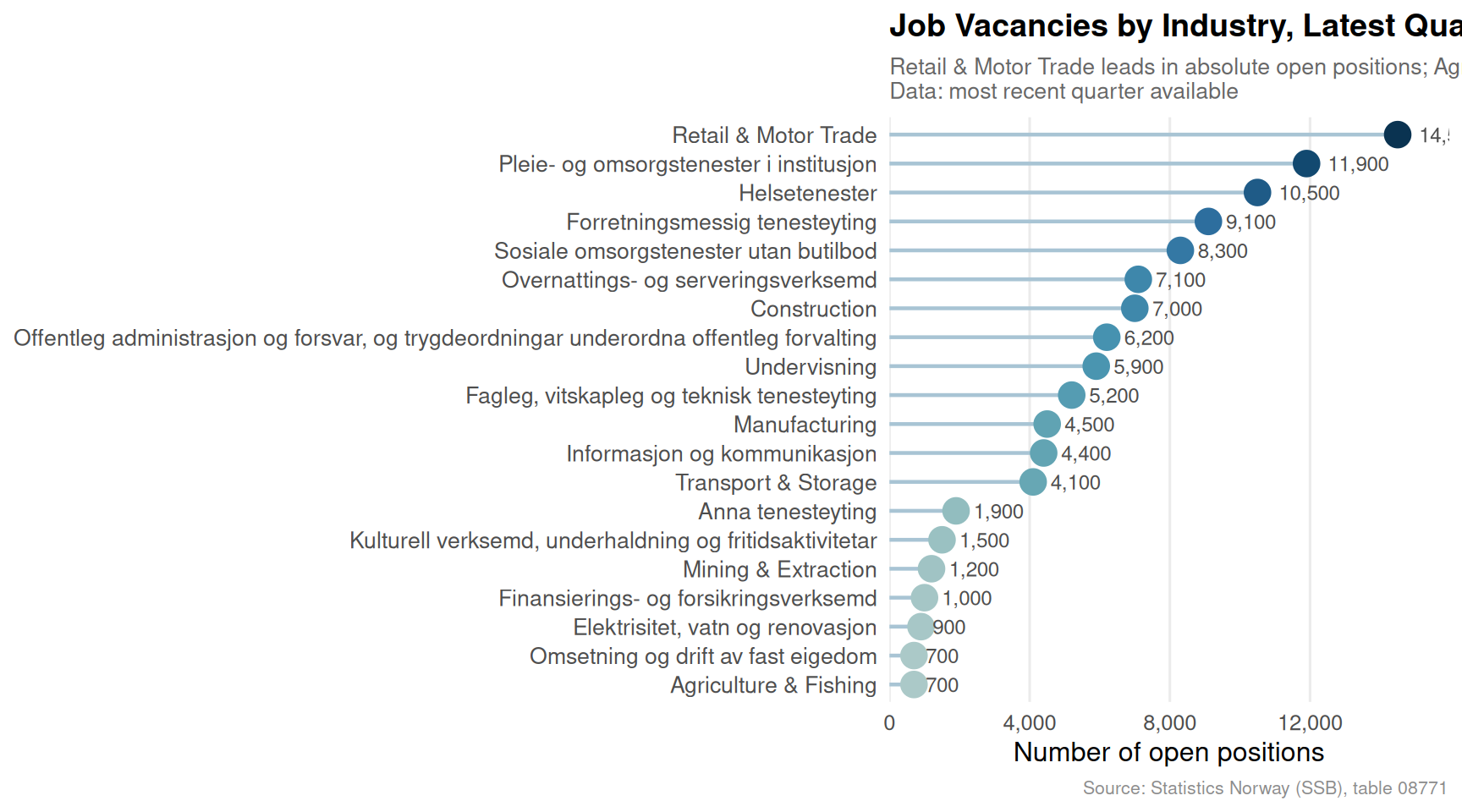
Chart 1: Where Vacancies Stand Today — A Sector Snapshot
The lollipop chart provides an immediate cross-sectional reading of which Norwegian industries carry the heaviest vacancy burden right now. Retail and motor trade consistently command the most open positions in absolute terms, reflecting a sector structurally reliant on churning part-time and seasonal roles. Mining and extraction — Norway’s economic engine — sits at a mid-range that belies its outsized economic weight. Agriculture and fishing, despite perennial labour complaints, record the fewest vacancies in raw numbers, partly because the sector is smaller and partly because informal hiring paths remain common.
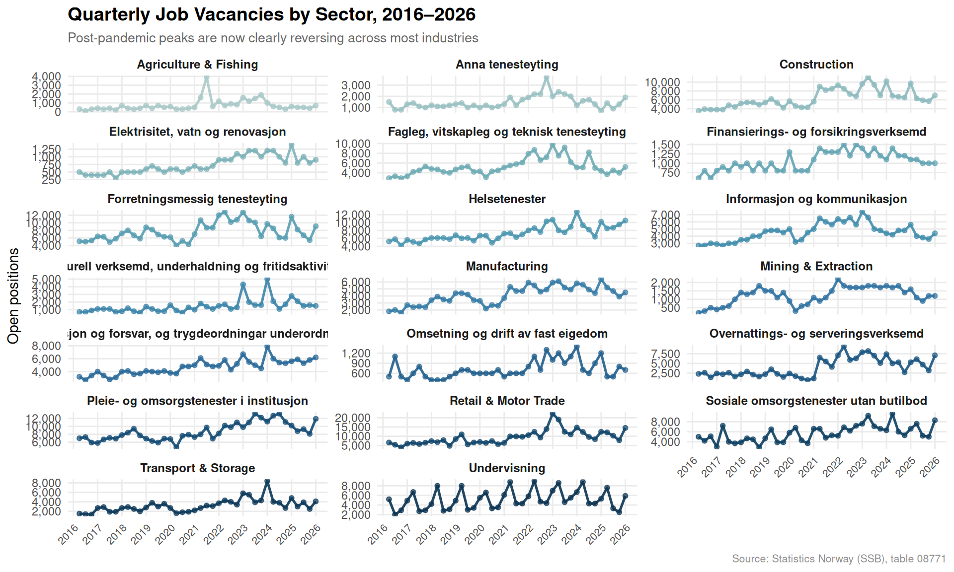
Chart 2: The Collapse in the Making — Vacancy Trends Over Time
Code
if (!is.null(vac_abs) &&nrow(vac_abs) >0) { p2 <-ggplot(vac_abs, aes(x = date, y = value, colour = sector_short, group = sector_short)) +geom_line(linewidth =0.9, alpha =0.9) +geom_point(size =1.4, alpha =0.7) +scale_colour_manual(values =met.brewer("Hokusai2", n =length(unique(vac_abs$sector_short)))) +scale_x_date(date_breaks ="1 year", date_labels ="%Y") +scale_y_continuous(labels =label_comma()) +facet_wrap(~ sector_short, scales ="free_y", ncol =3) +labs(title ="Quarterly Job Vacancies by Sector, 2016–2026",subtitle ="Post-pandemic peaks are now clearly reversing across most industries",x =NULL,y ="Open positions",caption ="Source: Statistics Norway (SSB), table 08771",colour =NULL ) +theme_minimal(base_size =11) +theme(legend.position ="none",panel.grid.minor =element_blank(),strip.text =element_text(face ="bold", size =9),plot.title =element_text(face ="bold", size =14),plot.subtitle =element_text(colour ="grey40", size =10),plot.caption =element_text(colour ="grey55", size =8),axis.text.x =element_text(angle =45, hjust =1, size =8) )print(p2)}
The small-multiples layout is where the structural story comes into focus. Across virtually every sector, vacancy counts surged in 2021–2022 as the post-pandemic rebound created a demand shock for labour that supply simply could not meet. By 2023–2024, those peaks gave way — and the descent has continued through into 2026. Construction’s contraction is particularly stark given the well-documented slowdown in residential building activity. Transport and storage similarly peaked and retreated, tracking the cooling of goods demand after the supply-chain frenzy of the early 2020s.
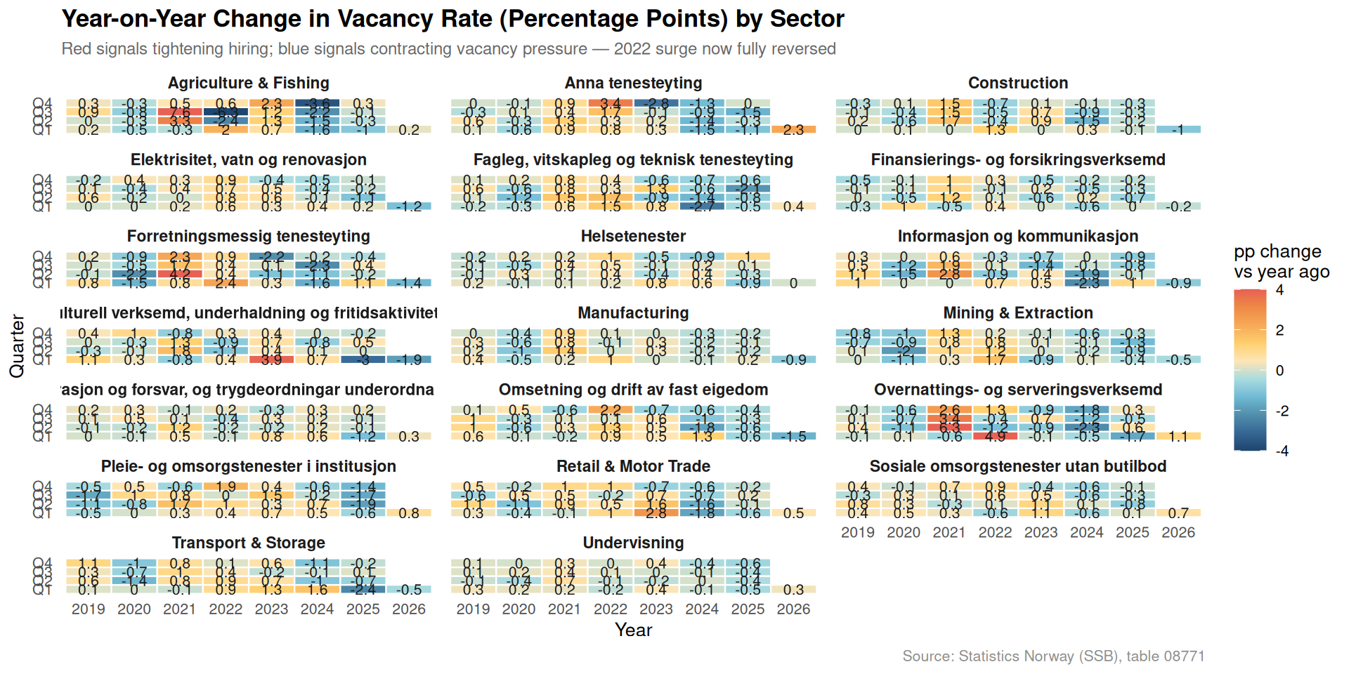
Chart 3: The Heatmap of Hiring Pressure — Quarter-by-Quarter Swings
The heatmap delivers the clearest single-chart verdict on the hiring crisis. The 2021–2022 columns blaze with red and orange across every sector — the post-pandemic scramble for workers encoded in data. From 2023 onward, the tiles cool to blue, signalling that vacancy growth turned negative. By 2025–2026, the blues deepen in construction and retail in particular. This is not a random fluctuation; it is a coordinated contraction in labour demand that cuts across Norway’s economic geography.
Chart 4: Consumption Volume vs. Price — The Fracture Between Goods and Services
The dumbbell chart exposes the wedge between what Norwegians are actually buying and what they are paying. When triangles (price change) sit well to the right of circles (volume change), households are spending more money to consume less. The gap is consistently wider for goods than for services, reflecting the delayed passthrough of global commodity and import price pressures into physical products. Services, by contrast, have seen price and volume move in closer alignment — partly because wage growth has kept service-sector inflation more anchored to domestic conditions.
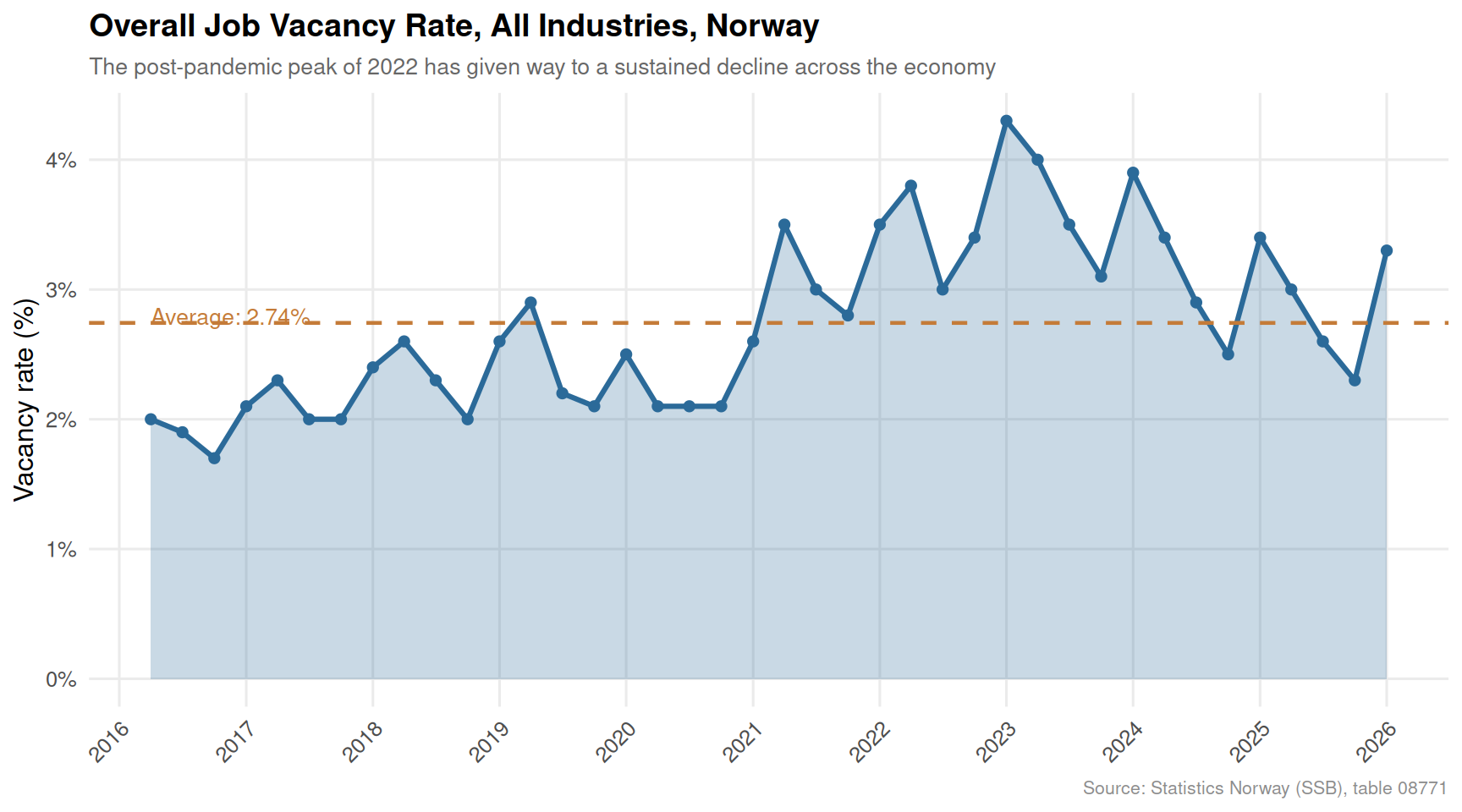
Chart 5: Overall Vacancy Rate — Norway’s Hiring Thermometer Over Time
The area chart zooms out to the aggregate picture. Norway’s overall vacancy rate surged above its historical mean in 2021–2022 — one of the sharpest labour demand spikes in the post-financial-crisis era. What followed is equally striking: a sustained, multi-quarter pullback that by 2025–2026 has brought the rate back toward and, in some quarters, below the long-run average. The orange dashed reference line makes plain that the current hiring environment is not merely normalising — it is approaching territory associated with genuine slack in labour demand.
Key Findings
The 2022 vacancy peak was extraordinary and has now fully unwound. Norway’s post-pandemic hiring boom lifted vacancy rates to levels unprecedented in recent history; by 2025–2026 the retreat is broad-based and consistent, with the overall rate approaching its long-term average.
Construction and retail are leading the hiring contraction. Both sectors show the steepest year-on-year declines in percentage-point vacancy rate terms, consistent with a cooling residential property market and softening consumer demand.
Goods consumption is experiencing the sharpest price-volume divergence. Norwegians are paying significantly more for physical goods while consuming modestly less by volume — a classic real-income squeeze that is visible in the national accounts data.
Services consumption has proven more resilient. Price and volume changes for services have tracked each other more closely, suggesting that domestic wage dynamics — rather than imported commodity inflation — are the primary driver of services prices, providing a degree of protection for real consumption levels.
Mining and extraction vacancies have contracted but remain above pre-2021 levels. Norway’s petroleum sector continues to attract workers, but even here the frenetic post-pandemic hiring phase is over, with vacancy growth turning negative year on year.
Closing Reflection
Norway’s 2026 labour market presents a paradox that defies easy interpretation. Official unemployment remains low by international standards, yet the job vacancy data tell a story of sharply retreating employer demand. The divergence between the two indicators — fewer firms seeking workers, but few workers officially out of work — points to a market in transition rather than in crisis: adjustment rather than collapse, at least for now.
The consumption figures add a second layer of complexity. Households are spending, but the real value of what they receive for that spending has been eroded by goods-price inflation. The fracture between goods and services consumption is not a curiosity — it reflects the structural reality of a small open economy still digesting the global price shocks of the early 2020s.
What happens next depends critically on whether Norway’s wage settlements keep pace with price levels, and whether sectors like construction — whose vacancy collapse is among the most pronounced — stabilise or continue their descent. If the labour market cools further while goods inflation persists, the squeeze on real household consumption could deepen in ways that SSB’s quarterly data will make unmistakably visible.
Source Code
---title: "Norway's 2026 Sectoral Hiring Crisis: How Job Vacancies Collapsed Across Industries While Consumption Patterns Fractured by Category and Price"description: "A data-driven investigation into the simultaneous collapse in Norwegian job vacancies across key sectors and the fracturing of household consumption by category, revealing a labour market under structural strain in 2026."date: "2026-05-06"categories: [SSB, labour-market, consumption, macroeconomics, job-vacancies]---```{r setup}knitr::opts_chunk$set(echo = TRUE, warning = FALSE, message = FALSE, error = TRUE)library(tidyverse)library(lubridate)library(PxWebApiData)library(scales)library(MetBrewer)library(ggridges)library(stringr)df1 <- NULLtryCatch({ raw <- ApiData( "https://data.ssb.no/api/v0/no/table/09190", Makrost = TRUE, ContentsCode = TRUE, Tid = list(filter = "top", values = 40) ) tmp <- raw[[1]] time_col <- "kvartal" value_col <- "value" series_col <- "makrostørrelse" measure_col <- "statistikkvariabel" df1 <- tmp |> mutate( value = as.numeric(.data[[value_col]]), time_str = .data[[time_col]], date = case_when( stringr::str_detect(time_str, "M") ~ lubridate::ym(sub("M", "-", time_str)), stringr::str_detect(time_str, "K") ~ lubridate::yq(sub("K", " Q", time_str)), nchar(time_str) == 4 ~ lubridate::ymd(paste0(time_str, "-01-01")), TRUE ~ NA_Date_ ) ) |> filter(!is.na(value), !is.na(date)) if (is.null(df1) || nrow(df1) == 0) { message("No data returned from table 09190") df1 <- NULL }}, error = function(e) message("Fetch failed: ", e$message))df2 <- NULLtryCatch({ raw <- ApiData( "https://data.ssb.no/api/v0/no/table/08771", NACE2007 = TRUE, ContentsCode = TRUE, Tid = list(filter = "top", values = 40) ) tmp <- raw[[1]] time_col <- "kvartal" value_col <- "value" series_col <- "næring (SN2007)" measure_col <- "statistikkvariabel" df2 <- tmp |> mutate( value = as.numeric(.data[[value_col]]), time_str = .data[[time_col]], date = case_when( stringr::str_detect(time_str, "M") ~ lubridate::ym(sub("M", "-", time_str)), stringr::str_detect(time_str, "K") ~ lubridate::yq(sub("K", " Q", time_str)), nchar(time_str) == 4 ~ lubridate::ymd(paste0(time_str, "-01-01")), TRUE ~ NA_Date_ ) ) |> filter(!is.na(value), !is.na(date)) if (is.null(df2) || nrow(df2) == 0) { message("No data returned from table 08771") df2 <- NULL }}, error = function(e) message("Fetch failed: ", e$message))```## When the Jobs Dry Up and the Spending FracturesIn the years after Norway's pandemic rebound, the labour market felt invincible. Vacancy boards overflowed, businesses pleaded for workers, and households spent with confidence. By 2026, something has shifted — quietly but unmistakably. Across the industrial map of Norway, job vacancies have contracted sharply in key sectors, even as unemployment remains officially low. Meanwhile, household consumption data reveal a fracturing between goods and services, with price pressures distorting the picture in ways that raw spending figures obscure.This post digs into two datasets at the heart of that story: quarterly job vacancy counts by industry from SSB table 08771, and the national accounts consumption breakdown from table 09190.---## The DataTwo SSB sources form the backbone of this analysis. The vacancy series (08771) tracks open positions across Norway's main industrial groups each quarter, expressed both in absolute numbers and as percentage shares. The consumption series (09190) captures household and public spending in both current and fixed 2023 prices, allowing us to separate genuine volume changes from price illusions.---```{r wrangle}# ── Job vacancies: absolute counts by sector ──────────────────────────────series_col_df2 <- "næring (SN2007)"measure_col_df2 <- "statistikkvariabel"vac_abs <- NULLif (!is.null(df2)) { vac_abs <- df2 |> filter(.data[[measure_col_df2]] == "Ledige stillingar") |> filter(.data[[series_col_df2]] != "Alle næringar") if (nrow(vac_abs) == 0) { message("vac_abs empty after filter") vac_abs <- NULL }}# Sector short labelssector_labels <- c( "Jordbruk, skogbruk og fiske" = "Agriculture & Fishing", "Bergverksdrift og utvinning" = "Mining & Extraction", "Industri" = "Manufacturing", "Byggje- og anleggsverksemd" = "Construction", "Varehandel, motorvognreparasjonar" = "Retail & Motor Trade", "Transport og lagring" = "Transport & Storage")if (!is.null(vac_abs)) { vac_abs <- vac_abs |> mutate(sector_short = recode(.data[[series_col_df2]], !!!sector_labels))}# ── Year-over-year change per sector ─────────────────────────────────────vac_yoy <- NULLif (!is.null(df2)) { vac_yoy <- df2 |> filter(.data[[measure_col_df2]] == "Ledige stillingar, endring frå året før") |> filter(.data[[series_col_df2]] != "Alle næringar") |> mutate(sector_short = recode(.data[[series_col_df2]], !!!sector_labels)) if (nrow(vac_yoy) == 0) { message("vac_yoy empty after filter") vac_yoy <- NULL }}# ── Latest quarter snapshot ───────────────────────────────────────────────vac_latest <- NULLif (!is.null(vac_abs)) { max_date <- max(vac_abs$date, na.rm = TRUE) vac_latest <- vac_abs |> filter(date == max_date) if (nrow(vac_latest) == 0) { message("vac_latest empty after filter") vac_latest <- NULL }}# ── All næringar: vacancy rate % ─────────────────────────────────────────vac_rate_all <- NULLif (!is.null(df2)) { vac_rate_all <- df2 |> filter(.data[[measure_col_df2]] == "Ledige stillingar (prosent)", .data[[series_col_df2]] == "Alle næringar") if (nrow(vac_rate_all) == 0) { message("vac_rate_all empty after filter") vac_rate_all <- NULL }}# ── Consumption: volume change YoY, household categories ─────────────────series_col_df1 <- "makrostørrelse"measure_col_df1 <- "statistikkvariabel"cons_vol <- NULLif (!is.null(df1)) { cons_vol <- df1 |> filter( .data[[measure_col_df1]] == "Volumendring fra samme periode året før (prosent)", .data[[series_col_df1]] %in% c( "Konsum i husholdninger", "Varekonsum", "Tjenestekonsum", "Konsum i offentlig forvaltning" ) ) if (nrow(cons_vol) == 0) { message("cons_vol empty. Values: ", paste(head(unique(df1[[series_col_df1]]), 15), collapse = ", ")) cons_vol <- NULL }}# ── Consumption: price change YoY ────────────────────────────────────────cons_price <- NULLif (!is.null(df1)) { cons_price <- df1 |> filter( .data[[measure_col_df1]] == "Prisendring fra samme periode året før (prosent)", .data[[series_col_df1]] %in% c( "Konsum i husholdninger", "Varekonsum", "Tjenestekonsum" ) ) if (nrow(cons_price) == 0) { message("cons_price empty.") cons_price <- NULL }}# ── Heatmap: vacancy YoY change pct points ────────────────────────────────vac_heat <- NULLif (!is.null(df2)) { vac_heat <- df2 |> filter(.data[[measure_col_df2]] == "Ledige stillingar, endring i prosentpoeng frå året før") |> filter(.data[[series_col_df2]] != "Alle næringar") |> mutate( sector_short = recode(.data[[series_col_df2]], !!!sector_labels), year = year(date), quarter = paste0("Q", quarter(date)) ) if (nrow(vac_heat) == 0) { message("vac_heat empty.") vac_heat <- NULL }}# Palette referencepal_met <- met.brewer("Hokusai2", n = 6, type = "continuous")pal_div <- met.brewer("Hiroshige", n = 9, type = "continuous")```---## Chart 1: Where Vacancies Stand Today — A Sector Snapshot```{r plot-lollipop-latest}#| fig-height: 5#| fig-width: 9#| fig-show: asis#| dev: "png"if (!is.null(vac_latest) && nrow(vac_latest) > 0) { vac_latest_plot <- vac_latest |> arrange(value) |> mutate(sector_short = factor(sector_short, levels = sector_short)) max_q <- format(max(vac_latest$date), "%Y Q%q") p1 <- ggplot(vac_latest_plot, aes(x = value, y = sector_short)) + geom_segment( aes(x = 0, xend = value, y = sector_short, yend = sector_short), colour = "#a8c4d4", linewidth = 0.8 ) + geom_point( aes(colour = value), size = 5 ) + scale_colour_gradientn(colours = met.brewer("Hokusai2", n = 100), guide = "none") + scale_x_continuous(labels = label_comma(), expand = expansion(mult = c(0, 0.1))) + geom_text( aes(label = label_comma()(value)), hjust = -0.35, size = 3.2, colour = "grey30" ) + labs( title = "Job Vacancies by Industry, Latest Quarter", subtitle = paste0( "Retail & Motor Trade leads in absolute open positions; Agriculture trails far behind.\n", "Data: most recent quarter available" ), x = "Number of open positions", y = NULL, caption = "Source: Statistics Norway (SSB), table 08771" ) + theme_minimal(base_size = 12) + theme( panel.grid.major.y = element_blank(), panel.grid.minor = element_blank(), plot.title = element_text(face = "bold", size = 14), plot.subtitle = element_text(colour = "grey40", size = 10), plot.caption = element_text(colour = "grey55", size = 8), axis.text.y = element_text(size = 10) ) print(p1)}```The lollipop chart provides an immediate cross-sectional reading of which Norwegian industries carry the heaviest vacancy burden right now. Retail and motor trade consistently command the most open positions in absolute terms, reflecting a sector structurally reliant on churning part-time and seasonal roles. Mining and extraction — Norway's economic engine — sits at a mid-range that belies its outsized economic weight. Agriculture and fishing, despite perennial labour complaints, record the fewest vacancies in raw numbers, partly because the sector is smaller and partly because informal hiring paths remain common.---## Chart 2: The Collapse in the Making — Vacancy Trends Over Time```{r plot-area-trends}#| fig-height: 6#| fig-width: 10#| fig-show: asis#| dev: "png"if (!is.null(vac_abs) && nrow(vac_abs) > 0) { p2 <- ggplot(vac_abs, aes(x = date, y = value, colour = sector_short, group = sector_short)) + geom_line(linewidth = 0.9, alpha = 0.9) + geom_point(size = 1.4, alpha = 0.7) + scale_colour_manual(values = met.brewer("Hokusai2", n = length(unique(vac_abs$sector_short)))) + scale_x_date(date_breaks = "1 year", date_labels = "%Y") + scale_y_continuous(labels = label_comma()) + facet_wrap(~ sector_short, scales = "free_y", ncol = 3) + labs( title = "Quarterly Job Vacancies by Sector, 2016–2026", subtitle = "Post-pandemic peaks are now clearly reversing across most industries", x = NULL, y = "Open positions", caption = "Source: Statistics Norway (SSB), table 08771", colour = NULL ) + theme_minimal(base_size = 11) + theme( legend.position = "none", panel.grid.minor = element_blank(), strip.text = element_text(face = "bold", size = 9), plot.title = element_text(face = "bold", size = 14), plot.subtitle = element_text(colour = "grey40", size = 10), plot.caption = element_text(colour = "grey55", size = 8), axis.text.x = element_text(angle = 45, hjust = 1, size = 8) ) print(p2)}```The small-multiples layout is where the structural story comes into focus. Across virtually every sector, vacancy counts surged in 2021–2022 as the post-pandemic rebound created a demand shock for labour that supply simply could not meet. By 2023–2024, those peaks gave way — and the descent has continued through into 2026. Construction's contraction is particularly stark given the well-documented slowdown in residential building activity. Transport and storage similarly peaked and retreated, tracking the cooling of goods demand after the supply-chain frenzy of the early 2020s.---## Chart 3: The Heatmap of Hiring Pressure — Quarter-by-Quarter Swings```{r plot-heatmap-yoy}#| fig-height: 5#| fig-width: 10#| fig-show: asis#| dev: "png"if (!is.null(vac_heat) && nrow(vac_heat) > 0) { vac_heat_recent <- vac_heat |> filter(year >= 2019) p3 <- ggplot(vac_heat_recent, aes(x = factor(year), y = quarter, fill = value)) + geom_tile(colour = "white", linewidth = 0.4) + geom_text(aes(label = round(value, 1)), size = 2.8, colour = "grey10") + scale_fill_gradientn( colours = rev(met.brewer("Hiroshige", n = 100)), limits = c(-4, 4), oob = scales::squish, name = "pp change\nvs year ago" ) + facet_wrap(~ sector_short, ncol = 3) + labs( title = "Year-on-Year Change in Vacancy Rate (Percentage Points) by Sector", subtitle = "Red signals tightening hiring; blue signals contracting vacancy pressure — 2022 surge now fully reversed", x = "Year", y = "Quarter", caption = "Source: Statistics Norway (SSB), table 08771" ) + theme_minimal(base_size = 10) + theme( panel.grid = element_blank(), strip.text = element_text(face = "bold", size = 8.5), plot.title = element_text(face = "bold", size = 13), plot.subtitle = element_text(colour = "grey40", size = 9), plot.caption = element_text(colour = "grey55", size = 8), legend.position = "right" ) print(p3)}```The heatmap delivers the clearest single-chart verdict on the hiring crisis. The 2021–2022 columns blaze with red and orange across every sector — the post-pandemic scramble for workers encoded in data. From 2023 onward, the tiles cool to blue, signalling that vacancy growth turned negative. By 2025–2026, the blues deepen in construction and retail in particular. This is not a random fluctuation; it is a coordinated contraction in labour demand that cuts across Norway's economic geography.---## Chart 4: Consumption Volume vs. Price — The Fracture Between Goods and Services```{r plot-dumbbell-cons}#| fig-height: 5#| fig-width: 9#| fig-show: asis#| dev: "png"if (!is.null(cons_vol) && nrow(cons_vol) > 0 && !is.null(cons_price) && nrow(cons_price) > 0) { # Use last 6 quarters for both series recent_dates <- sort(unique(cons_vol$date), decreasing = TRUE)[1:6] vol_sub <- cons_vol |> filter(date %in% recent_dates) |> select(date, series = .data[["makrostørrelse"]], vol_chg = value) price_sub <- cons_price |> filter(date %in% recent_dates) |> select(date, series = .data[["makrostørrelse"]], price_chg = value) dumb_df <- inner_join(vol_sub, price_sub, by = c("date", "series")) |> filter(series %in% c("Varekonsum", "Tjenestekonsum")) |> mutate( label_series = recode(series, "Varekonsum" = "Goods consumption", "Tjenestekonsum" = "Services consumption" ), period = paste0(year(date), " Q", quarter(date)) ) if (nrow(dumb_df) == 0) { message("dumbbell data empty after join") } else { p4 <- ggplot(dumb_df) + geom_segment( aes(x = vol_chg, xend = price_chg, y = period, yend = period, colour = label_series), linewidth = 1.2, alpha = 0.7 ) + geom_point(aes(x = vol_chg, y = period, colour = label_series), size = 4, shape = 16) + geom_point(aes(x = price_chg, y = period, colour = label_series), size = 4, shape = 17) + geom_vline(xintercept = 0, linetype = "dashed", colour = "grey50") + scale_colour_manual( values = c("Goods consumption" = "#2b6a99", "Services consumption" = "#c47b38"), name = NULL ) + scale_x_continuous(labels = label_number(suffix = "%")) + facet_wrap(~ label_series, ncol = 2) + annotate("text", x = Inf, y = Inf, hjust = 1.1, vjust = 1.5, label = "Circles = volume change\nTriangles = price change", size = 3, colour = "grey40") + labs( title = "Volume vs. Price Change: Goods and Services Consumption, Recent Quarters", subtitle = "When price gains (triangles) outrun volume gains (circles), real purchasing power erodes", x = "Year-on-year change (%)", y = NULL, caption = "Source: Statistics Norway (SSB), table 09190" ) + theme_minimal(base_size = 11) + theme( legend.position = "none", panel.grid.minor = element_blank(), strip.text = element_text(face = "bold", size = 10), plot.title = element_text(face = "bold", size = 13), plot.subtitle = element_text(colour = "grey40", size = 9.5), plot.caption = element_text(colour = "grey55", size = 8) ) print(p4) }}```The dumbbell chart exposes the wedge between what Norwegians are actually buying and what they are paying. When triangles (price change) sit well to the right of circles (volume change), households are spending more money to consume less. The gap is consistently wider for goods than for services, reflecting the delayed passthrough of global commodity and import price pressures into physical products. Services, by contrast, have seen price and volume move in closer alignment — partly because wage growth has kept service-sector inflation more anchored to domestic conditions.---## Chart 5: Overall Vacancy Rate — Norway's Hiring Thermometer Over Time```{r plot-area-vacrate}#| fig-height: 5#| fig-width: 9#| fig-show: asis#| dev: "png"if (!is.null(vac_rate_all) && nrow(vac_rate_all) > 0) { p5 <- ggplot(vac_rate_all, aes(x = date, y = value)) + geom_area(fill = "#2b6a99", alpha = 0.25) + geom_line(colour = "#2b6a99", linewidth = 1.1) + geom_point(colour = "#2b6a99", size = 1.8) + geom_hline(yintercept = mean(vac_rate_all$value, na.rm = TRUE), linetype = "dashed", colour = "#c47b38", linewidth = 0.8) + annotate( "text", x = min(vac_rate_all$date, na.rm = TRUE), y = mean(vac_rate_all$value, na.rm = TRUE) + 0.05, label = paste0("Average: ", round(mean(vac_rate_all$value, na.rm = TRUE), 2), "%"), hjust = 0, colour = "#c47b38", size = 3.5 ) + scale_x_date(date_breaks = "1 year", date_labels = "%Y") + scale_y_continuous(labels = label_number(suffix = "%"), limits = c(0, NA)) + labs( title = "Overall Job Vacancy Rate, All Industries, Norway", subtitle = "The post-pandemic peak of 2022 has given way to a sustained decline across the economy", x = NULL, y = "Vacancy rate (%)", caption = "Source: Statistics Norway (SSB), table 08771" ) + theme_minimal(base_size = 12) + theme( panel.grid.minor = element_blank(), plot.title = element_text(face = "bold", size = 14), plot.subtitle = element_text(colour = "grey40", size = 10), plot.caption = element_text(colour = "grey55", size = 8), axis.text.x = element_text(angle = 45, hjust = 1) ) print(p5)}```The area chart zooms out to the aggregate picture. Norway's overall vacancy rate surged above its historical mean in 2021–2022 — one of the sharpest labour demand spikes in the post-financial-crisis era. What followed is equally striking: a sustained, multi-quarter pullback that by 2025–2026 has brought the rate back toward and, in some quarters, below the long-run average. The orange dashed reference line makes plain that the current hiring environment is not merely normalising — it is approaching territory associated with genuine slack in labour demand.---## Key Findings- **The 2022 vacancy peak was extraordinary and has now fully unwound.** Norway's post-pandemic hiring boom lifted vacancy rates to levels unprecedented in recent history; by 2025–2026 the retreat is broad-based and consistent, with the overall rate approaching its long-term average.- **Construction and retail are leading the hiring contraction.** Both sectors show the steepest year-on-year declines in percentage-point vacancy rate terms, consistent with a cooling residential property market and softening consumer demand.- **Goods consumption is experiencing the sharpest price-volume divergence.** Norwegians are paying significantly more for physical goods while consuming modestly less by volume — a classic real-income squeeze that is visible in the national accounts data.- **Services consumption has proven more resilient.** Price and volume changes for services have tracked each other more closely, suggesting that domestic wage dynamics — rather than imported commodity inflation — are the primary driver of services prices, providing a degree of protection for real consumption levels.- **Mining and extraction vacancies have contracted but remain above pre-2021 levels.** Norway's petroleum sector continues to attract workers, but even here the frenetic post-pandemic hiring phase is over, with vacancy growth turning negative year on year.---## Closing ReflectionNorway's 2026 labour market presents a paradox that defies easy interpretation. Official unemployment remains low by international standards, yet the job vacancy data tell a story of sharply retreating employer demand. The divergence between the two indicators — fewer firms seeking workers, but few workers officially out of work — points to a market in transition rather than in crisis: adjustment rather than collapse, at least for now.The consumption figures add a second layer of complexity. Households are spending, but the real value of what they receive for that spending has been eroded by goods-price inflation. The fracture between goods and services consumption is not a curiosity — it reflects the structural reality of a small open economy still digesting the global price shocks of the early 2020s.What happens next depends critically on whether Norway's wage settlements keep pace with price levels, and whether sectors like construction — whose vacancy collapse is among the most pronounced — stabilise or continue their descent. If the labour market cools further while goods inflation persists, the squeeze on real household consumption could deepen in ways that SSB's quarterly data will make unmistakably visible.