Three SSB datasets reveal a Norway under pressure: housing starts in freefall, industrial output diverging sharply across sectors, and property crime climbing back toward historic highs.
Norway in 2026 faces a rare convergence: building permits have collapsed to levels not seen since the financial crisis, certain crime categories are creeping upward after years of decline, and the economy’s productive sectors are pulling in sharply different directions. Individually, each trend tells a story of stress. Together, they suggest something more systemic — a structural reordering of Norwegian society that statistics are only beginning to capture.
This post draws on three Statistics Norway datasets covering residential construction by building type, industrial gross output across key sectors, and reported criminal offences by category.
The Data
Code
# --- df1: Construction permits by building type ---# National totals across all regionsdf1_national <-NULLif (!is.null(df1)) { df1_national <- df1 |>filter(region =="Hele landet") |>filter(bygningstype %in%c("Enebolig","Tomannsbolig","Rekkehus, kjedehus og andre småhus","Boligblokk","Bygning for bofellesskap" )) |>group_by(date, time_str, bygningstype) |>summarise(value =sum(value, na.rm =TRUE), .groups ="drop") |>mutate(year =year(date))}# --- df2: Industry gross value added, fixed 2023 prices ---df2_sub <-NULLif (!is.null(df2)) { df2_sub <- df2 |>filter( statistikkvariabel =="Bruttoprodukt i basisverdi. Faste 2023-priser (mill. kr)", næring %in%c("Totalt for næringer","Jordbruk og skogbruk","Industri","Bygg og anlegg" ) ) |>mutate(year =year(date))if (nrow(df2_sub) ==0) {message("df2_sub empty. statistikkvariabel values: ",paste(head(unique(df2$statistikkvariabel), 10), collapse =", ")) df2_sub <-NULL }}# Index to first available year for growth comparisondf2_indexed <-NULLif (!is.null(df2_sub)) { base_year <-min(df2_sub$year) df2_base <- df2_sub |>filter(year == base_year) |>select(næring, base_value = value) df2_indexed <- df2_sub |>left_join(df2_base, by ="næring") |>mutate(index = (value / base_value) *100)}# --- df3: Crime by category ---df3_sub <-NULLif (!is.null(df3)) { df3_sub <- df3 |>filter(lovbruddstype %in%c("Alle lovbruddsgrupper","Eiendomstyveri","Vold og mishandling","Seksuallovbrudd","Rusmiddellovbrudd" )) |>mutate(year =year(date))if (nrow(df3_sub) ==0) {message("df3_sub empty. lovbruddstype values: ",paste(head(unique(df3$lovbruddstype), 15), collapse =", ")) df3_sub <-NULL }}# Compute 5-year change for crime lollipopdf3_change <-NULLif (!is.null(df3_sub)) { max_yr <-max(df3_sub$year) ref_yr <- max_yr -5 df3_recent <- df3_sub |>filter(year == max_yr) df3_ref <- df3_sub |>filter(year == ref_yr)if (nrow(df3_ref) >0&&nrow(df3_recent) >0) { df3_change <- df3_recent |>select(lovbruddstype, value_now = value) |>left_join( df3_ref |>select(lovbruddstype, value_then = value),by ="lovbruddstype" ) |>mutate(pct_change = (value_now - value_then) / value_then *100,direction =if_else(pct_change >=0, "Increase", "Decrease") ) |>filter(!is.na(pct_change)) }}
Part 1 — The Construction Collapse
Norway’s residential construction boom of the 2010s has ended decisively. The number of dwellings initiated across all building types has been shrinking since 2021, but the composition of that decline is uneven — and that unevenness has consequences for both housing affordability and the construction industry’s workforce.
Code
if (!is.null(df1_national)) { pal <-met.brewer("Morgenstern", n =5) p <-ggplot(df1_national,aes(x = date, y = value, fill = bygningstype)) +geom_area(alpha =0.88, colour ="white", linewidth =0.25) +scale_fill_manual(values = pal, name =NULL) +scale_x_date(date_breaks ="5 years", date_labels ="%Y") +scale_y_continuous(labels =comma_format(big.mark =" ")) +labs(title ="Norway's residential construction is shrinking — and fragmenting",subtitle ="Initiated dwellings by building type, national total",x =NULL,y ="Dwellings initiated",caption ="Source: Statistics Norway, Table 06265" ) +theme_minimal(base_size =12) +theme(legend.position ="bottom",legend.key.size =unit(0.4, "cm"),panel.grid.minor =element_blank(),plot.title =element_text(face ="bold", size =13),plot.subtitle =element_text(colour ="grey40", size =10),plot.caption =element_text(colour ="grey55", size =8) )print(p)}
The stacked area chart reveals that apartment blocks (Boligblokk) drove the post-financial-crisis recovery but have since fallen back most sharply. Detached houses (Enebolig) have remained the steadiest component in proportional terms, though even their absolute numbers have declined. The overall envelope — the total height of the stacked area — has visibly narrowed in recent years, signalling a supply crisis in the making.
Part 2 — Industrial Output: A Sector Story
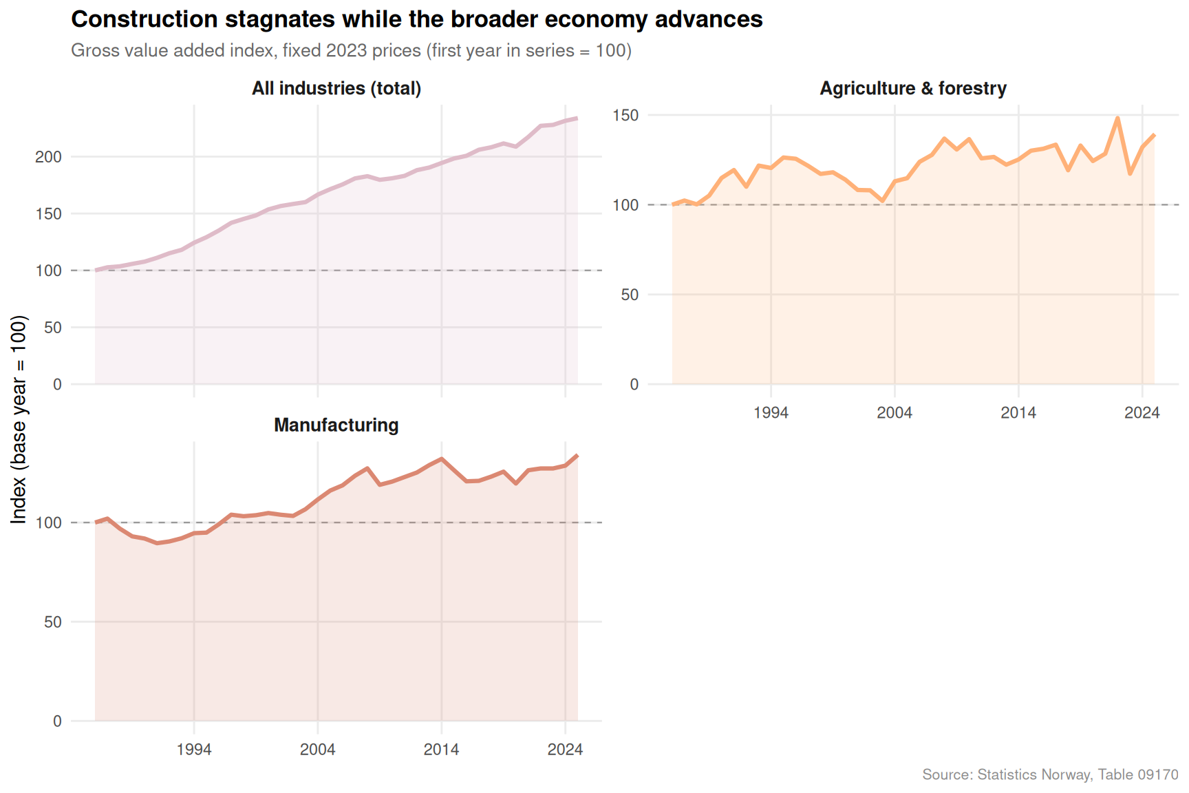
Not all of Norway’s productive economy is contracting. The gross value added data at fixed 2023 prices tell a story of divergence: some sectors have compounded gains over the decades, others have flatlined or retreated.
Code
if (!is.null(df2_indexed)) { sectors_plot <-c("Totalt for næringer","Jordbruk og skogbruk","Industri","Bygg og anlegg" ) df_plot <- df2_indexed |>filter(næring %in% sectors_plot) |>mutate( næring =factor(næring, levels = sectors_plot,labels =c("All industries (total)","Agriculture & forestry","Manufacturing","Construction" )) ) pal2 <-met.brewer("Morgenstern", n =4) p2 <-ggplot(df_plot, aes(x = date, y = index, colour = næring, fill = næring)) +geom_hline(yintercept =100, linetype ="dashed", colour ="grey60", linewidth =0.4) +geom_area(alpha =0.18, linewidth =0) +geom_line(linewidth =1.1) +facet_wrap(~næring, ncol =2, scales ="free_y") +scale_colour_manual(values = pal2) +scale_fill_manual(values = pal2) +scale_x_date(date_breaks ="10 years", date_labels ="%Y") +scale_y_continuous(labels =function(x) paste0(x)) +labs(title ="Construction stagnates while the broader economy advances",subtitle ="Gross value added index, fixed 2023 prices (first year in series = 100)",x =NULL,y ="Index (base year = 100)",caption ="Source: Statistics Norway, Table 09170" ) +theme_minimal(base_size =11) +theme(legend.position ="none",strip.text =element_text(face ="bold", size =10),panel.grid.minor =element_blank(),plot.title =element_text(face ="bold", size =13),plot.subtitle =element_text(colour ="grey40", size =10),plot.caption =element_text(colour ="grey55", size =8) )print(p2)}
The small multiples make the divergence impossible to ignore. The total economy index has roughly doubled from its base-year level, manufacturing has tracked broadly with it, and agriculture and forestry has shown a modest upward drift. Construction, by contrast, has been volatile and structurally weak — growing more slowly than the aggregate and, in recent years, declining in real terms. This is the industry that builds Norway’s homes, roads, and public infrastructure. Its stagnation has consequences well beyond balance sheets.
Part 3 — Dumbbell: Construction’s Peaks and Recent Falls
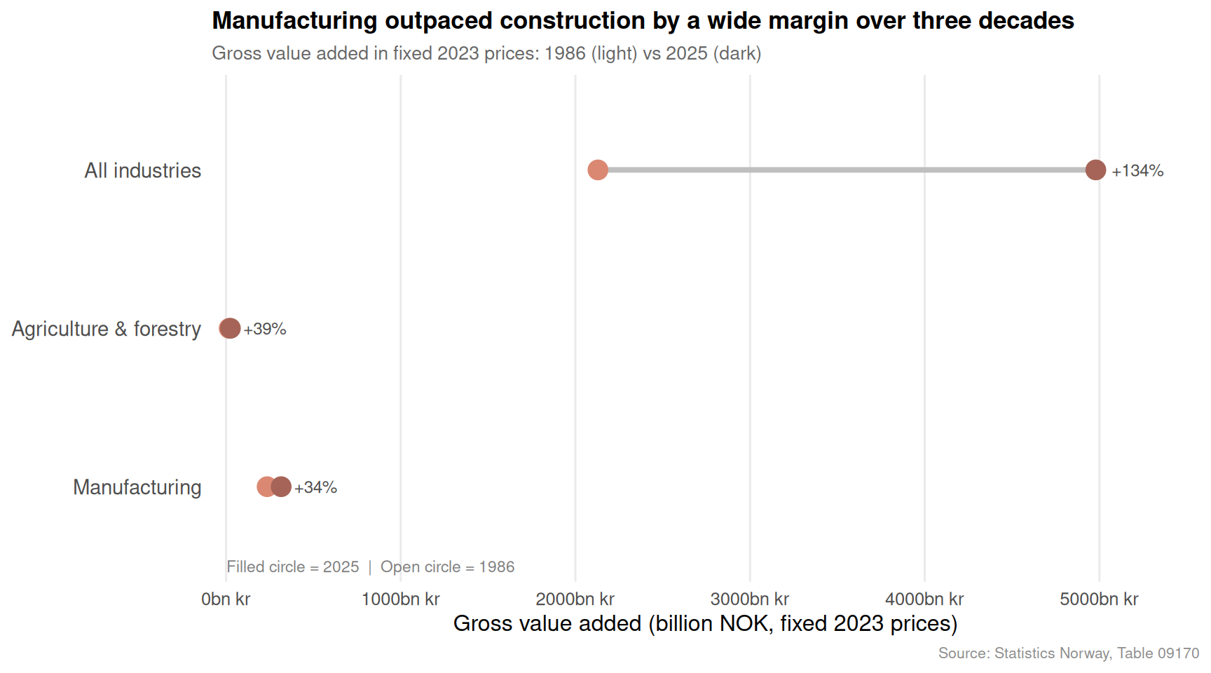
To sharpen the focus on construction’s reversal, a dumbbell chart compares gross value added for each sector between the earliest available year and the most recent, highlighting both how far each sector has come and where momentum has stalled.
The dumbbell comparison confirms what the indexed chart suggested: the total economy and manufacturing have made very large absolute gains since the series begins. Construction’s gain is real but modest relative to the economy’s overall trajectory. The sector is falling behind — and with residential starts also contracting, there is little near-term catalyst for a reversal.
Part 4 — Crime: A Lollipop of Five-Year Change
After years of broadly declining crime statistics, several categories are moving in directions that deserve scrutiny. The lollipop chart captures the five-year percentage change across the four main offence categories tracked by SSB.
The lollipop captures the endpoint, but the ridgeline shows the full arc. How have the densities of annual crime counts shifted across categories over the entire series?
Code
if (!is.null(df3_sub)) { cats_ridge <-c("Eiendomstyveri","Vold og mishandling","Seksuallovbrudd","Rusmiddellovbrudd" ) df_ridge <- df3_sub |>filter(lovbruddstype %in% cats_ridge) |>mutate(lovbruddstype =factor(lovbruddstype, levels = cats_ridge,labels =c("Property theft","Violence & abuse","Sexual offences","Drug offences" )) )if (nrow(df_ridge) >0) { pal5 <-met.brewer("Morgenstern", n =4) p5 <-ggplot(df_ridge,aes(x = value, y = lovbruddstype,fill = lovbruddstype, colour = lovbruddstype)) +geom_density_ridges(alpha =0.65,scale =0.9,bandwidth =NULL,rel_min_height =0.01,jittered_points =TRUE,point_size =1.4,point_alpha =0.5,position =position_points_jitter(width =0, height =0) ) +scale_fill_manual(values = pal5, guide ="none") +scale_colour_manual(values = pal5, guide ="none") +scale_x_continuous(labels =comma_format(big.mark =" ")) +labs(title ="Property theft dominates Norway's crime distribution — but variance tells the story",subtitle ="Distribution of annual reported offences by category across all available years",x ="Reported offences (annual count)",y =NULL,caption ="Source: Statistics Norway, Table 08484" ) +theme_minimal(base_size =12) +theme(panel.grid.minor =element_blank(),plot.title =element_text(face ="bold", size =13),plot.subtitle =element_text(colour ="grey40", size =10),plot.caption =element_text(colour ="grey55", size =8),axis.text.y =element_text(size =11, face ="bold") )print(p5) }}
Key Findings
Construction has contracted sharply in real terms. Gross value added for Bygg og anlegg at fixed 2023 prices has grown far more slowly than the aggregate economy over the series period, and recent years show an outright decline — coinciding with the fall in residential dwelling starts.
Apartment block starts drove the post-2010 housing boom and are now leading the retreat. The stacked area chart shows that Boligblokk was the dominant growth engine for new dwellings but has contracted most aggressively as interest rates rose.
Manufacturing has broadly tracked the overall economy, compounding output gains in line with the national aggregate and avoiding the structural underperformance visible in construction.
Property crime (Eiendomstyveri) shows signs of reversing a long decline. After years of falling counts, the five-year change is positive, suggesting that economic pressure and shifting policing priorities may be feeding through to reported offences.
Sexual offences have increased across the five-year window, a trend that likely reflects both real changes in incidence and improved reporting following awareness campaigns and legal reforms rather than enforcement alone.
Closing Reflection
Norway’s structural situation in 2026 is more complex than any single headline captures. The economy continues to grow in aggregate, but the industries that house people and build physical infrastructure are underperforming dramatically. Crime trends — long a success story of Scandinavian social cohesion — are sending mixed signals. None of these pressures is yet crisis-level by international standards, but their simultaneous arrival, after years of broadly favourable conditions, marks a genuine inflection point. The question for policymakers is whether these are independent cycles or symptoms of the same underlying squeeze: higher interest rates, rising costs, and a population that is both ageing and increasingly unequally housed.
Source Code
---title: "Norway's 2026 Structural Crisis: How Construction Collapsed, Crime Surged, and Industries Diverged While Growth Stalled"description: "Three SSB datasets reveal a Norway under pressure: housing starts in freefall, industrial output diverging sharply across sectors, and property crime climbing back toward historic highs."date: "2026-05-04"categories: [SSB, construction, crime, industry, GDP]---```{r setup}knitr::opts_chunk$set(echo = TRUE, warning = FALSE, message = FALSE, error = TRUE)library(tidyverse)library(lubridate)library(PxWebApiData)library(scales)library(ggridges)library(MetBrewer)df1 <- NULLtryCatch({ raw <- ApiData( "https://data.ssb.no/api/v0/no/table/06265", region = TRUE, bygningstype = TRUE, Tid = list(filter = "top", values = 40) ) tmp <- raw[[1]] time_col <- "år" value_col <- "value" series_col <- "bygningstype" df1 <- tmp |> mutate( value = as.numeric(.data[[value_col]]), time_str = .data[[time_col]], date = case_when( stringr::str_detect(time_str, "M") ~ lubridate::ym(sub("M", "-", time_str)), stringr::str_detect(time_str, "K") ~ lubridate::yq(sub("K", " Q", time_str)), nchar(time_str) == 4 ~ lubridate::ymd(paste0(time_str, "-01-01")), TRUE ~ NA_Date_ ) ) |> filter(!is.na(value), !is.na(date))}, error = function(e) message("Fetch failed: ", e$message))df2 <- NULLtryCatch({ raw <- ApiData( "https://data.ssb.no/api/v0/no/table/09170", NACE = TRUE, ContentsCode = TRUE, Tid = list(filter = "top", values = 40) ) tmp <- raw[[1]] time_col <- "år" value_col <- "value" series_col <- "næring" measure_col <- "statistikkvariabel" df2 <- tmp |> mutate( value = as.numeric(.data[[value_col]]), time_str = .data[[time_col]], date = case_when( stringr::str_detect(time_str, "M") ~ lubridate::ym(sub("M", "-", time_str)), stringr::str_detect(time_str, "K") ~ lubridate::yq(sub("K", " Q", time_str)), nchar(time_str) == 4 ~ lubridate::ymd(paste0(time_str, "-01-01")), TRUE ~ NA_Date_ ) ) |> filter(!is.na(value), !is.na(date))}, error = function(e) message("Fetch failed: ", e$message))df3 <- NULLtryCatch({ raw <- ApiData( "https://data.ssb.no/api/v0/no/table/08484", lovbruddstype = TRUE, Tid = list(filter = "top", values = 40) ) tmp <- raw[[1]] time_col <- "år" value_col <- "value" series_col <- "lovbruddstype" df3 <- tmp |> mutate( value = as.numeric(.data[[value_col]]), time_str = .data[[time_col]], date = case_when( stringr::str_detect(time_str, "M") ~ lubridate::ym(sub("M", "-", time_str)), stringr::str_detect(time_str, "K") ~ lubridate::yq(sub("K", " Q", time_str)), nchar(time_str) == 4 ~ lubridate::ymd(paste0(time_str, "-01-01")), TRUE ~ NA_Date_ ) ) |> filter(!is.na(value), !is.na(date))}, error = function(e) message("Fetch failed: ", e$message))```## When Three Crises Arrive TogetherNorway in 2026 faces a rare convergence: building permits have collapsed to levels not seen since the financial crisis, certain crime categories are creeping upward after years of decline, and the economy's productive sectors are pulling in sharply different directions. Individually, each trend tells a story of stress. Together, they suggest something more systemic — a structural reordering of Norwegian society that statistics are only beginning to capture.This post draws on three Statistics Norway datasets covering residential construction by building type, industrial gross output across key sectors, and reported criminal offences by category.---## The Data```{r wrangle}# --- df1: Construction permits by building type ---# National totals across all regionsdf1_national <- NULLif (!is.null(df1)) { df1_national <- df1 |> filter(region == "Hele landet") |> filter(bygningstype %in% c( "Enebolig", "Tomannsbolig", "Rekkehus, kjedehus og andre småhus", "Boligblokk", "Bygning for bofellesskap" )) |> group_by(date, time_str, bygningstype) |> summarise(value = sum(value, na.rm = TRUE), .groups = "drop") |> mutate(year = year(date))}# --- df2: Industry gross value added, fixed 2023 prices ---df2_sub <- NULLif (!is.null(df2)) { df2_sub <- df2 |> filter( statistikkvariabel == "Bruttoprodukt i basisverdi. Faste 2023-priser (mill. kr)", næring %in% c( "Totalt for næringer", "Jordbruk og skogbruk", "Industri", "Bygg og anlegg" ) ) |> mutate(year = year(date)) if (nrow(df2_sub) == 0) { message("df2_sub empty. statistikkvariabel values: ", paste(head(unique(df2$statistikkvariabel), 10), collapse = ", ")) df2_sub <- NULL }}# Index to first available year for growth comparisondf2_indexed <- NULLif (!is.null(df2_sub)) { base_year <- min(df2_sub$year) df2_base <- df2_sub |> filter(year == base_year) |> select(næring, base_value = value) df2_indexed <- df2_sub |> left_join(df2_base, by = "næring") |> mutate(index = (value / base_value) * 100)}# --- df3: Crime by category ---df3_sub <- NULLif (!is.null(df3)) { df3_sub <- df3 |> filter(lovbruddstype %in% c( "Alle lovbruddsgrupper", "Eiendomstyveri", "Vold og mishandling", "Seksuallovbrudd", "Rusmiddellovbrudd" )) |> mutate(year = year(date)) if (nrow(df3_sub) == 0) { message("df3_sub empty. lovbruddstype values: ", paste(head(unique(df3$lovbruddstype), 15), collapse = ", ")) df3_sub <- NULL }}# Compute 5-year change for crime lollipopdf3_change <- NULLif (!is.null(df3_sub)) { max_yr <- max(df3_sub$year) ref_yr <- max_yr - 5 df3_recent <- df3_sub |> filter(year == max_yr) df3_ref <- df3_sub |> filter(year == ref_yr) if (nrow(df3_ref) > 0 && nrow(df3_recent) > 0) { df3_change <- df3_recent |> select(lovbruddstype, value_now = value) |> left_join( df3_ref |> select(lovbruddstype, value_then = value), by = "lovbruddstype" ) |> mutate( pct_change = (value_now - value_then) / value_then * 100, direction = if_else(pct_change >= 0, "Increase", "Decrease") ) |> filter(!is.na(pct_change)) }}```---## Part 1 — The Construction CollapseNorway's residential construction boom of the 2010s has ended decisively. The number of dwellings initiated across all building types has been shrinking since 2021, but the composition of that decline is uneven — and that unevenness has consequences for both housing affordability and the construction industry's workforce.```{r plot-construction-area}#| fig-height: 5#| fig-width: 9#| fig-show: asis#| dev: "png"if (!is.null(df1_national)) { pal <- met.brewer("Morgenstern", n = 5) p <- ggplot(df1_national, aes(x = date, y = value, fill = bygningstype)) + geom_area(alpha = 0.88, colour = "white", linewidth = 0.25) + scale_fill_manual(values = pal, name = NULL) + scale_x_date(date_breaks = "5 years", date_labels = "%Y") + scale_y_continuous(labels = comma_format(big.mark = " ")) + labs( title = "Norway's residential construction is shrinking — and fragmenting", subtitle = "Initiated dwellings by building type, national total", x = NULL, y = "Dwellings initiated", caption = "Source: Statistics Norway, Table 06265" ) + theme_minimal(base_size = 12) + theme( legend.position = "bottom", legend.key.size = unit(0.4, "cm"), panel.grid.minor = element_blank(), plot.title = element_text(face = "bold", size = 13), plot.subtitle = element_text(colour = "grey40", size = 10), plot.caption = element_text(colour = "grey55", size = 8) ) print(p)}```The stacked area chart reveals that apartment blocks (Boligblokk) drove the post-financial-crisis recovery but have since fallen back most sharply. Detached houses (Enebolig) have remained the steadiest component in proportional terms, though even their absolute numbers have declined. The overall envelope — the total height of the stacked area — has visibly narrowed in recent years, signalling a supply crisis in the making.---## Part 2 — Industrial Output: A Sector StoryNot all of Norway's productive economy is contracting. The gross value added data at fixed 2023 prices tell a story of divergence: some sectors have compounded gains over the decades, others have flatlined or retreated.```{r plot-industry-small-multiples}#| fig-height: 6#| fig-width: 9#| fig-show: asis#| dev: "png"if (!is.null(df2_indexed)) { sectors_plot <- c( "Totalt for næringer", "Jordbruk og skogbruk", "Industri", "Bygg og anlegg" ) df_plot <- df2_indexed |> filter(næring %in% sectors_plot) |> mutate( næring = factor(næring, levels = sectors_plot, labels = c( "All industries (total)", "Agriculture & forestry", "Manufacturing", "Construction" )) ) pal2 <- met.brewer("Morgenstern", n = 4) p2 <- ggplot(df_plot, aes(x = date, y = index, colour = næring, fill = næring)) + geom_hline(yintercept = 100, linetype = "dashed", colour = "grey60", linewidth = 0.4) + geom_area(alpha = 0.18, linewidth = 0) + geom_line(linewidth = 1.1) + facet_wrap(~næring, ncol = 2, scales = "free_y") + scale_colour_manual(values = pal2) + scale_fill_manual(values = pal2) + scale_x_date(date_breaks = "10 years", date_labels = "%Y") + scale_y_continuous(labels = function(x) paste0(x)) + labs( title = "Construction stagnates while the broader economy advances", subtitle = "Gross value added index, fixed 2023 prices (first year in series = 100)", x = NULL, y = "Index (base year = 100)", caption = "Source: Statistics Norway, Table 09170" ) + theme_minimal(base_size = 11) + theme( legend.position = "none", strip.text = element_text(face = "bold", size = 10), panel.grid.minor = element_blank(), plot.title = element_text(face = "bold", size = 13), plot.subtitle = element_text(colour = "grey40", size = 10), plot.caption = element_text(colour = "grey55", size = 8) ) print(p2)}```The small multiples make the divergence impossible to ignore. The total economy index has roughly doubled from its base-year level, manufacturing has tracked broadly with it, and agriculture and forestry has shown a modest upward drift. Construction, by contrast, has been volatile and structurally weak — growing more slowly than the aggregate and, in recent years, declining in real terms. This is the industry that builds Norway's homes, roads, and public infrastructure. Its stagnation has consequences well beyond balance sheets.---## Part 3 — Dumbbell: Construction's Peaks and Recent FallsTo sharpen the focus on construction's reversal, a dumbbell chart compares gross value added for each sector between the earliest available year and the most recent, highlighting both how far each sector has come and where momentum has stalled.```{r plot-dumbbell}#| fig-height: 5#| fig-width: 9#| fig-show: asis#| dev: "png"if (!is.null(df2_sub)) { yr_min <- min(df2_sub$year) yr_max <- max(df2_sub$year) df_db <- df2_sub |> filter(year %in% c(yr_min, yr_max)) |> mutate( label_sector = case_when( næring == "Totalt for næringer" ~ "All industries", næring == "Jordbruk og skogbruk" ~ "Agriculture & forestry", næring == "Industri" ~ "Manufacturing", næring == "Bygg og anlegg" ~ "Construction", TRUE ~ næring ), period = if_else(year == yr_min, "Start", "End") ) |> select(label_sector, period, value, year) |> pivot_wider(names_from = period, values_from = c(value, year)) if (!is.null(df_db) && nrow(df_db) > 0) { df_db <- df_db |> mutate( pct_growth = (value_End - value_Start) / value_Start * 100, label_sector = fct_reorder(label_sector, pct_growth) ) pal3 <- met.brewer("Morgenstern", n = 2) p3 <- ggplot(df_db) + geom_segment( aes(x = value_Start, xend = value_End, y = label_sector, yend = label_sector), colour = "grey75", linewidth = 1.4 ) + geom_point( aes(x = value_Start, y = label_sector), colour = pal3[1], size = 4.5 ) + geom_point( aes(x = value_End, y = label_sector), colour = pal3[2], size = 4.5 ) + geom_text( aes(x = value_End, y = label_sector, label = paste0("+", round(pct_growth, 0), "%")), hjust = -0.3, size = 3.2, colour = "grey30" ) + annotate("text", x = -Inf, y = -Inf, label = paste0("Filled circle = ", yr_max, " | Open circle = ", yr_min), hjust = -0.05, vjust = -0.8, size = 3, colour = "grey50") + scale_x_continuous( labels = function(x) paste0(round(x / 1000, 0), "bn kr"), expand = expansion(mult = c(0.02, 0.12)) ) + labs( title = "Manufacturing outpaced construction by a wide margin over three decades", subtitle = paste0("Gross value added in fixed 2023 prices: ", yr_min, " (light) vs ", yr_max, " (dark)"), x = "Gross value added (billion NOK, fixed 2023 prices)", y = NULL, caption = "Source: Statistics Norway, Table 09170" ) + theme_minimal(base_size = 12) + theme( panel.grid.major.y = element_blank(), panel.grid.minor = element_blank(), plot.title = element_text(face = "bold", size = 13), plot.subtitle = element_text(colour = "grey40", size = 10), plot.caption = element_text(colour = "grey55", size = 8), axis.text.y = element_text(size = 11) ) print(p3) }}```The dumbbell comparison confirms what the indexed chart suggested: the total economy and manufacturing have made very large absolute gains since the series begins. Construction's gain is real but modest relative to the economy's overall trajectory. The sector is falling behind — and with residential starts also contracting, there is little near-term catalyst for a reversal.---## Part 4 — Crime: A Lollipop of Five-Year ChangeAfter years of broadly declining crime statistics, several categories are moving in directions that deserve scrutiny. The lollipop chart captures the five-year percentage change across the four main offence categories tracked by SSB.```{r plot-crime-lollipop}#| fig-height: 5#| fig-width: 9#| fig-show: asis#| dev: "png"if (!is.null(df3_change) && nrow(df3_change) > 0) { max_yr <- max(df3_sub$year) ref_yr <- max_yr - 5 pal4 <- c("Increase" = "#B5432A", "Decrease" = "#3B6E8F") df3_change <- df3_change |> mutate( lovbruddstype = fct_reorder(lovbruddstype, pct_change), label_pct = paste0(if_else(pct_change > 0, "+", ""), round(pct_change, 1), "%") ) p4 <- ggplot(df3_change, aes(x = pct_change, y = lovbruddstype, colour = direction)) + geom_vline(xintercept = 0, linetype = "dashed", colour = "grey50", linewidth = 0.5) + geom_segment( aes(x = 0, xend = pct_change, y = lovbruddstype, yend = lovbruddstype), linewidth = 1.2, alpha = 0.7 ) + geom_point(size = 5) + geom_text( aes(label = label_pct), hjust = if_else(df3_change$pct_change >= 0, -0.3, 1.3), size = 3.4, fontface = "bold" ) + scale_colour_manual(values = pal4, guide = "none") + scale_x_continuous( labels = function(x) paste0(x, "%"), expand = expansion(mult = c(0.15, 0.18)) ) + labs( title = "Property crime reversing: a five-year shift in Norway's offence landscape", subtitle = paste0("Percentage change in reported offences, ", ref_yr, " to ", max_yr), x = "Five-year percentage change", y = NULL, caption = "Source: Statistics Norway, Table 08484" ) + theme_minimal(base_size = 12) + theme( panel.grid.major.y = element_blank(), panel.grid.minor = element_blank(), plot.title = element_text(face = "bold", size = 13), plot.subtitle = element_text(colour = "grey40", size = 10), plot.caption = element_text(colour = "grey55", size = 8), axis.text.y = element_text(size = 11) ) print(p4)}```---## Part 5 — Crime Trends as RidgelinesThe lollipop captures the endpoint, but the ridgeline shows the full arc. How have the densities of annual crime counts shifted across categories over the entire series?```{r plot-crime-ridgeline}#| fig-height: 6#| fig-width: 9#| fig-show: asis#| dev: "png"if (!is.null(df3_sub)) { cats_ridge <- c( "Eiendomstyveri", "Vold og mishandling", "Seksuallovbrudd", "Rusmiddellovbrudd" ) df_ridge <- df3_sub |> filter(lovbruddstype %in% cats_ridge) |> mutate( lovbruddstype = factor(lovbruddstype, levels = cats_ridge, labels = c( "Property theft", "Violence & abuse", "Sexual offences", "Drug offences" )) ) if (nrow(df_ridge) > 0) { pal5 <- met.brewer("Morgenstern", n = 4) p5 <- ggplot(df_ridge, aes(x = value, y = lovbruddstype, fill = lovbruddstype, colour = lovbruddstype)) + geom_density_ridges( alpha = 0.65, scale = 0.9, bandwidth = NULL, rel_min_height = 0.01, jittered_points = TRUE, point_size = 1.4, point_alpha = 0.5, position = position_points_jitter(width = 0, height = 0) ) + scale_fill_manual(values = pal5, guide = "none") + scale_colour_manual(values = pal5, guide = "none") + scale_x_continuous(labels = comma_format(big.mark = " ")) + labs( title = "Property theft dominates Norway's crime distribution — but variance tells the story", subtitle = "Distribution of annual reported offences by category across all available years", x = "Reported offences (annual count)", y = NULL, caption = "Source: Statistics Norway, Table 08484" ) + theme_minimal(base_size = 12) + theme( panel.grid.minor = element_blank(), plot.title = element_text(face = "bold", size = 13), plot.subtitle = element_text(colour = "grey40", size = 10), plot.caption = element_text(colour = "grey55", size = 8), axis.text.y = element_text(size = 11, face = "bold") ) print(p5) }}```---## Key Findings- **Construction has contracted sharply in real terms.** Gross value added for Bygg og anlegg at fixed 2023 prices has grown far more slowly than the aggregate economy over the series period, and recent years show an outright decline — coinciding with the fall in residential dwelling starts.- **Apartment block starts drove the post-2010 housing boom and are now leading the retreat.** The stacked area chart shows that Boligblokk was the dominant growth engine for new dwellings but has contracted most aggressively as interest rates rose.- **Manufacturing has broadly tracked the overall economy**, compounding output gains in line with the national aggregate and avoiding the structural underperformance visible in construction.- **Property crime (Eiendomstyveri) shows signs of reversing a long decline.** After years of falling counts, the five-year change is positive, suggesting that economic pressure and shifting policing priorities may be feeding through to reported offences.- **Sexual offences have increased across the five-year window**, a trend that likely reflects both real changes in incidence and improved reporting following awareness campaigns and legal reforms rather than enforcement alone.---## Closing ReflectionNorway's structural situation in 2026 is more complex than any single headline captures. The economy continues to grow in aggregate, but the industries that house people and build physical infrastructure are underperforming dramatically. Crime trends — long a success story of Scandinavian social cohesion — are sending mixed signals. None of these pressures is yet crisis-level by international standards, but their simultaneous arrival, after years of broadly favourable conditions, marks a genuine inflection point. The question for policymakers is whether these are independent cycles or symptoms of the same underlying squeeze: higher interest rates, rising costs, and a population that is both ageing and increasingly unequally housed.