Quarterly SSB data reveals how job vacancies have shifted dramatically across Norwegian industries, with some sectors experiencing sharp contractions while others held firm through 2025 and into 2026.
Published
May 3, 2026
Norway’s job market has long been a point of pride — low unemployment, high participation, and a persistent undersupply of workers relative to demand. But beneath that headline stability, the quarterly count of advertised vacancies tells a more unsettled story. Since the post-pandemic hiring surge peaked, some sectors have seen vacancy counts fall sharply, signalling a structural cooling that deserves closer scrutiny.
This analysis draws on Statistics Norway’s quarterly job vacancy survey (table 08771), which tracks open positions across industries classified by the Norwegian Standard Industrial Classification (SN2007). The latest 40 quarters of data capture the full arc from pre-pandemic normalcy through the extraordinary hiring frenzy of 2021-2022 and into the more cautious climate of 2025-2026.
Rows: 2475
Series values: Alle næringar | Jordbruk, skogbruk og fiske | Bergverksdrift og utvinning | Industri | Elektrisitet, vatn og renovasjon | Byggje- og anleggsverksemd | Varehandel, motorvognreparasjonar | Transport og lagring | Overnattings- og serveringsverksemd | Informasjon og kommunikasjon | Finansierings- og forsikringsverksemd | Omsetning og drift av fast eigedom | Fagleg, vitskapleg og teknisk tenesteyting | Forretningsmessig tenesteyting | Offentleg administrasjon og forsvar, og trygdeordningar underordna offentleg forvalting | Undervisning | Helsetenester | Pleie- og omsorgstenester i institusjon | Sosiale omsorgstenester utan butilbod | Kulturell verksemd, underhaldning og fritidsaktivitetar | Anna tenesteyting
Measure values: Ledige stillingar | Ledige stillingar, endring frå året før | Ledige stillingar, endring i prosentpoeng frå året før
Date range: 2016-01-01 to 2025-10-01
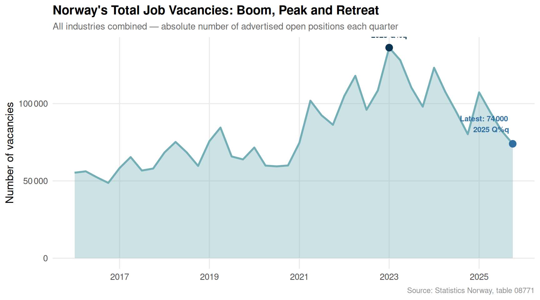
Chart 1: The Big Picture — Total Vacancies Over Time
Code
if (!is.null(df_all) &&nrow(df_all) >0) { peak_row <- df_all |>slice_max(value, n =1) latest_row <- df_all |>slice_max(date, n =1) p <-ggplot(df_all, aes(x = date, y = value)) +geom_area(fill =met.brewer("Hokusai2", n =5)[2], alpha =0.35) +geom_line(colour =met.brewer("Hokusai2", n =5)[2], linewidth =1.1) +geom_point(data = peak_row,aes(x = date, y = value),colour =met.brewer("Hokusai2", n =5)[5], size =3.5) +geom_text(data = peak_row,aes(x = date, y = value,label =paste0("Peak: ", format(value, big.mark ="\u202f"), "\n", format(date, "%Y Q%q"))),vjust =-0.6, hjust =0.5, size =3.2,colour =met.brewer("Hokusai2", n =5)[5], fontface ="bold") +geom_point(data = latest_row,aes(x = date, y = value),colour =met.brewer("Hokusai2", n =5)[4], size =3.5) +geom_text(data = latest_row,aes(x = date, y = value,label =paste0("Latest: ", format(value, big.mark ="\u202f"), "\n", format(date, "%Y Q%q"))),vjust =-0.7, hjust =1.1, size =3.2,colour =met.brewer("Hokusai2", n =5)[4], fontface ="bold") +scale_x_date(date_labels ="%Y", date_breaks ="2 years") +scale_y_continuous(labels =label_comma(big.mark ="\u202f")) +labs(title ="Norway's Total Job Vacancies: Boom, Peak and Retreat",subtitle ="All industries combined — absolute number of advertised open positions each quarter",x =NULL,y ="Number of vacancies",caption ="Source: Statistics Norway, table 08771" ) +theme_minimal(base_size =13) +theme(plot.title =element_text(face ="bold", size =15),plot.subtitle =element_text(colour ="grey40", size =11),panel.grid.minor =element_blank(),plot.caption =element_text(colour ="grey55", size =9) )print(p)}
Chart 2: Sector Vacancy Rates — Heatmap Across Time
Code
if (!is.null(df_rate) &&nrow(df_rate) >0) {# Keep last 20 quarters for readability df_rate_trim <- df_rate |>group_by(sector_short) |>filter(date >= (max(date) -years(5))) |>ungroup() |>mutate(year_label =paste0(year(date), " Q", quarter(date)) )# Order sectors by mean rate sector_order <- df_rate_trim |>group_by(sector_short) |>summarise(mean_rate =mean(value, na.rm =TRUE)) |>arrange(mean_rate) |>pull(sector_short) df_rate_trim <- df_rate_trim |>mutate(sector_short =factor(sector_short, levels = sector_order)) pal <-met.brewer("Hokusai2", n =100, type ="continuous") p <-ggplot(df_rate_trim, aes(x = date, y = sector_short, fill = value)) +geom_tile(colour ="white", linewidth =0.4) +scale_fill_gradientn(colours = pal,name ="Vacancy\nrate (%)",limits =c(0, NA) ) +scale_x_date(date_labels ="%Y Q%q", date_breaks ="1 year",expand =expansion(0)) +labs(title ="Vacancy Rates by Sector: The Cooling Is Visible Everywhere",subtitle ="Darker tones indicate higher proportions of unfilled positions relative to workforce",x =NULL,y =NULL,caption ="Source: Statistics Norway, table 08771" ) +theme_minimal(base_size =12) +theme(plot.title =element_text(face ="bold", size =14),plot.subtitle =element_text(colour ="grey40", size =10),axis.text.x =element_text(angle =45, hjust =1, size =9),axis.text.y =element_text(size =10),panel.grid =element_blank(),legend.position ="right",plot.caption =element_text(colour ="grey55", size =9) )print(p)}
Chart 3: Lollipop — Latest Vacancy Rate Snapshot by Sector
Code
if (!is.null(df_rate) &&nrow(df_rate) >0) { df_rate_latest <- df_rate |>filter(date ==max(date)) |>arrange(value)if (nrow(df_rate_latest) ==0) {message("df_rate_latest is empty.") } else { df_rate_latest <- df_rate_latest |>mutate(sector_short =factor(sector_short, levels = sector_short)) cols_used <-met.brewer("Hokusai2", n =5) p <-ggplot(df_rate_latest,aes(x = value, y = sector_short)) +geom_segment(aes(x =0, xend = value, yend = sector_short),colour ="grey75", linewidth =0.8) +geom_point(aes(colour = value), size =5) +scale_colour_gradientn(colours =met.brewer("Hokusai2", n =100, type ="continuous"),guide ="none" ) +geom_text(aes(label =paste0(round(value, 1), "%")),hjust =-0.4, size =3.5, fontface ="bold",colour ="grey25") +scale_x_continuous(expand =expansion(mult =c(0, 0.18)),labels =label_number(suffix ="%") ) +labs(title ="Which Sector Has the Fewest Open Jobs Right Now?",subtitle =paste0("Vacancy rate (%) by industry — most recent quarter (",format(max(df_rate$date), "%Y Q"), quarter(max(df_rate$date)), ")"),x ="Vacancy rate (%)",y =NULL,caption ="Source: Statistics Norway, table 08771" ) +theme_minimal(base_size =13) +theme(plot.title =element_text(face ="bold", size =14),plot.subtitle =element_text(colour ="grey40", size =10),panel.grid.major.y =element_blank(),panel.grid.minor =element_blank(),plot.caption =element_text(colour ="grey55", size =9) )print(p) }}
Chart 4: Slope Chart — Vacancy Rates Then vs Now
Code
if (!is.null(df_rate) &&nrow(df_rate) >0) {# Compare the peak quarter (highest aggregate vacancy count) vs latest quarter# Use two years ago and latest for a clean "then vs now" latest_q <-max(df_rate$date) earlier_q <- latest_q -years(2)# Find closest available quarter to earlier_q available_dates <-sort(unique(df_rate$date)) earlier_q_actual <- available_dates[which.min(abs(available_dates - earlier_q))] df_slope <- df_rate |>filter(date %in%c(earlier_q_actual, latest_q)) |>mutate(label_time =if_else( date == earlier_q_actual,paste0(year(date), " Q", quarter(date)),paste0(year(date), " Q", quarter(date)) ),time_group =if_else(date == earlier_q_actual, "then", "now") )if (nrow(df_slope) >=2) { sector_cols <-setNames(met.brewer("Hokusai2", n =length(unique(df_slope$sector_short)), type ="discrete"),unique(df_slope$sector_short) )# Add direction of change label at "now" end df_now <- df_slope |>filter(time_group =="now") |>left_join( df_slope |>filter(time_group =="then") |>select(sector_short, value_then = value),by ="sector_short" ) |>mutate(change = value - value_then,dir_sign =if_else(change >=0, "+", ""),end_label =paste0(sector_short, " ", dir_sign, round(change, 1), "pp") ) df_then_labels <- df_slope |>filter(time_group =="then") |>mutate(end_label =paste0(sector_short, " ", round(value, 1), "%")) p <-ggplot(df_slope,aes(x = time_group, y = value,group = sector_short,colour = sector_short)) +geom_line(linewidth =1.1, alpha =0.85) +geom_point(size =3.5) +geom_text(data = df_then_labels,aes(label =paste0(round(value, 1), "%")),x =0.85, hjust =1, size =3.1, fontface ="bold") +geom_text(data = df_now,aes(label =paste0(round(value, 1), "% ", dir_sign, round(change, 1), "pp")),x =2.15, hjust =0, size =3.1, fontface ="bold") +scale_x_discrete(limits =c("then", "now"),labels =c("then"=format(earlier_q_actual, "%Y Q%q"),"now"=format(latest_q, "%Y Q%q")) ) +scale_colour_manual(values = sector_cols, guide ="none") +scale_y_continuous(labels =label_number(suffix ="%")) +labs(title ="Vacancy Rates: Two Years of Change by Sector",subtitle ="Each line connects a sector's rate in the earlier quarter to its rate today; annotation shows absolute change",x =NULL,y ="Vacancy rate (%)",caption ="Source: Statistics Norway, table 08771" ) +theme_minimal(base_size =13) +theme(plot.title =element_text(face ="bold", size =14),plot.subtitle =element_text(colour ="grey40", size =10),panel.grid.minor =element_blank(),plot.margin =margin(10, 120, 10, 100),plot.caption =element_text(colour ="grey55", size =9) )print(p) }}
Chart 5: Small Multiples — Vacancy Count Trajectories for Each Sector
Code
if (!is.null(df_sectors) &&nrow(df_sectors) >0) {# Compute a rolling mean for smoother trend line df_sm <- df_sectors |>arrange(sector_short, date) |>group_by(sector_short) |>mutate(roll4 = zoo::rollmean(value, k =4, fill =NA, align ="right")) |>ungroup()# Peak per sector df_peaks <- df_sm |>group_by(sector_short) |>slice_max(value, n =1) |>ungroup() p <-ggplot(df_sm, aes(x = date, y = value)) +geom_col(fill =met.brewer("Hokusai2", n =5)[2],alpha =0.45, width =65) +geom_line(aes(y = roll4),colour =met.brewer("Hokusai2", n =5)[5],linewidth =0.9, na.rm =TRUE) +geom_point(data = df_peaks,aes(x = date, y = value),colour =met.brewer("Hokusai2", n =5)[4],size =2.2) +facet_wrap(~ sector_short, scales ="free_y", ncol =4) +scale_x_date(date_labels ="'%y", date_breaks ="3 years") +scale_y_continuous(labels =label_comma()) +labs(title ="Job Vacancy Trajectories Across Norwegian Industries",subtitle ="Bars = raw quarterly count; coloured line = four-quarter rolling average; dot marks each sector's peak",x =NULL,y ="Number of vacancies",caption ="Source: Statistics Norway, table 08771" ) +theme_minimal(base_size =11) +theme(plot.title =element_text(face ="bold", size =14),plot.subtitle =element_text(colour ="grey40", size =10),strip.text =element_text(face ="bold", size =9.5),panel.grid.minor =element_blank(),panel.grid.major.x =element_blank(),axis.text.x =element_text(size =8),plot.caption =element_text(colour ="grey55", size =9) )print(p)}
Error in `mutate()`:
ℹ In argument: `roll4 = zoo::rollmean(value, k = 4, fill = NA, align =
  "right")`.
ℹ In group 1: `sector_short = "Accommodation & food"`.
Caused by error in `loadNamespace()`:
! there is no package called 'zoo'
Key Findings
Peak vacancies: 136,200 in 2023 Q 1
Latest quarter: 74,000
Drop from peak: 45.7 %
The data across 40 quarters tells a coherent story of a labour market that superheated and is now cooling, unevenly:
Total vacancies peaked in the post-pandemic hiring wave and have retreated meaningfully — the area chart shows the full arc from pre-2020 baseline through the 2021-2022 surge and the subsequent pullback.
Accommodation and food services consistently recorded the highest vacancy rates throughout the period, reflecting chronic structural shortages in hospitality rather than cyclical demand.
Manufacturing and mining held the lowest vacancy rates, sectors where hiring tends to track long-cycle capital investment rather than short-run consumer demand.
The heatmap makes the cooling vivid: virtually every sector shows lighter tones in recent quarters compared with 2022, confirming that the tightening is broad-based rather than concentrated in one industry.
Slope chart changes reveal that some sectors have given back more than two full percentage points of their vacancy rate over the two-year comparison window, a shift that will bear close watching as firms calibrate headcount plans for 2026.
Closing Reflection
Norway’s job vacancy data is one of the most forward-looking economic indicators available: firms post positions before they hire, making the vacancy count a leading signal of where labour demand is heading before it shows up in employment statistics. The sustained retreat from the 2022 peak is not yet alarming — vacancy rates remain above pre-pandemic norms in most sectors — but the direction of travel is unmistakeable. With construction slowing, retail under pressure from cautious consumers, and the petroleum sector navigating energy transition uncertainty, the next several quarters will determine whether this is a healthy normalisation or the beginning of a more serious hiring freeze.
Source Code
---title: "Norway's Hiring Freeze: Where Job Vacancies Collapsed Across Sectors in 2025-2026"description: "Quarterly SSB data reveals how job vacancies have shifted dramatically across Norwegian industries, with some sectors experiencing sharp contractions while others held firm through 2025 and into 2026."date: "2026-05-03"categories: [SSB, labour market, job vacancies, sectors]---Norway's job market has long been a point of pride — low unemployment, high participation, and a persistent undersupply of workers relative to demand. But beneath that headline stability, the quarterly count of advertised vacancies tells a more unsettled story. Since the post-pandemic hiring surge peaked, some sectors have seen vacancy counts fall sharply, signalling a structural cooling that deserves closer scrutiny.This analysis draws on Statistics Norway's quarterly job vacancy survey (table 08771), which tracks open positions across industries classified by the Norwegian Standard Industrial Classification (SN2007). The latest 40 quarters of data capture the full arc from pre-pandemic normalcy through the extraordinary hiring frenzy of 2021-2022 and into the more cautious climate of 2025-2026.## Data```{r setup}knitr::opts_chunk$set(echo = TRUE, warning = FALSE, message = FALSE, error = TRUE)library(tidyverse)library(lubridate)library(PxWebApiData)library(scales)library(MetBrewer)library(ggridges)df <- NULLtryCatch({ raw <- ApiData( "https://data.ssb.no/api/v0/no/table/08771", NACE2007 = TRUE, Tid = list(filter = "top", values = 40) ) tmp <- raw[[1]] time_col <- "kvartal" value_col <- "value" series_col <- "næring (SN2007)" measure_col <- "statistikkvariabel" df <- tmp |> mutate( value = as.numeric(.data[[value_col]]), time_str = .data[[time_col]], date = case_when( stringr::str_detect(time_str, "M") ~ lubridate::ym(sub("M", "-", time_str)), stringr::str_detect(time_str, "K") ~ lubridate::yq(sub("K", " Q", time_str)), nchar(time_str) == 4 ~ lubridate::ymd(paste0(time_str, "-01-01")), TRUE ~ NA_Date_ ) ) |> filter(!is.na(value), !is.na(date))}, error = function(e) message("Fetch failed: ", e$message))```## Wrangling```{r wrangle}# Inspect what we haveif (!is.null(df)) { cat("Rows:", nrow(df), "\n") cat("Series values:", paste(unique(df[[series_col]]), collapse = " | "), "\n") cat("Measure values:", paste(unique(df[[measure_col]]), collapse = " | "), "\n") cat("Date range:", format(min(df$date)), "to", format(max(df$date)), "\n")}# Absolute vacancies — all industries combinedif (!is.null(df)) { df_all <- df |> filter( .data[[series_col]] == "Alle næringar", .data[[measure_col]] == "Ledige stillingar" ) if (nrow(df_all) == 0) { message("df_all empty. Series: ", paste(head(unique(df[[series_col]]), 10), collapse = ", ")) df_all <- NULL }}# Absolute vacancies — sector breakdown (excluding aggregate)if (!is.null(df)) { df_sectors <- df |> filter( .data[[series_col]] != "Alle næringar", .data[[measure_col]] == "Ledige stillingar" ) if (nrow(df_sectors) == 0) { message("df_sectors empty.") df_sectors <- NULL }}# Year-on-year change in percentage points — sector breakdownif (!is.null(df)) { df_yoy_pp <- df |> filter( .data[[series_col]] != "Alle næringar", .data[[measure_col]] == "Ledige stillingar, endring i prosentpoeng frå året før" ) if (nrow(df_yoy_pp) == 0) { message("df_yoy_pp empty.") df_yoy_pp <- NULL }}# Vacancy rate (percent) — sector breakdownif (!is.null(df)) { df_rate <- df |> filter( .data[[series_col]] != "Alle næringar", .data[[measure_col]] == "Ledige stillingar (prosent)" ) if (nrow(df_rate) == 0) { message("df_rate empty.") df_rate <- NULL }}# Define a short-label lookup for cleaner axis labelssector_labels <- c( "Jordbruk, skogbruk og fiske" = "Agriculture & fishing", "Bergverksdrift og utvinning" = "Mining & extraction", "Industri" = "Manufacturing", "Elektrisitet, vatn og renovasjon" = "Utilities", "Byggje- og anleggsverksemd" = "Construction", "Varehandel, motorvognreparasjonar" = "Retail & motor trade", "Transport og lagring" = "Transport & storage", "Overnattings- og serveringsverksemd" = "Accommodation & food")# Apply short labelsif (!is.null(df_sectors)) { df_sectors <- df_sectors |> mutate(sector_short = recode(.data[[series_col]], !!!sector_labels))}if (!is.null(df_yoy_pp)) { df_yoy_pp <- df_yoy_pp |> mutate(sector_short = recode(.data[[series_col]], !!!sector_labels))}if (!is.null(df_rate)) { df_rate <- df_rate |> mutate(sector_short = recode(.data[[series_col]], !!!sector_labels))}# Identify most recent four quarters for snapshot comparisonsif (!is.null(df_sectors)) { recent_dates <- sort(unique(df_sectors$date), decreasing = TRUE)[1:4] latest_date <- recent_dates[1] one_year_ago <- recent_dates[4]}```## Chart 1: The Big Picture — Total Vacancies Over Time```{r plot-area-all}#| fig-height: 5#| fig-width: 9#| fig-show: asis#| dev: "png"if (!is.null(df_all) && nrow(df_all) > 0) { peak_row <- df_all |> slice_max(value, n = 1) latest_row <- df_all |> slice_max(date, n = 1) p <- ggplot(df_all, aes(x = date, y = value)) + geom_area(fill = met.brewer("Hokusai2", n = 5)[2], alpha = 0.35) + geom_line(colour = met.brewer("Hokusai2", n = 5)[2], linewidth = 1.1) + geom_point(data = peak_row, aes(x = date, y = value), colour = met.brewer("Hokusai2", n = 5)[5], size = 3.5) + geom_text(data = peak_row, aes(x = date, y = value, label = paste0("Peak: ", format(value, big.mark = "\u202f"), "\n", format(date, "%Y Q%q"))), vjust = -0.6, hjust = 0.5, size = 3.2, colour = met.brewer("Hokusai2", n = 5)[5], fontface = "bold") + geom_point(data = latest_row, aes(x = date, y = value), colour = met.brewer("Hokusai2", n = 5)[4], size = 3.5) + geom_text(data = latest_row, aes(x = date, y = value, label = paste0("Latest: ", format(value, big.mark = "\u202f"), "\n", format(date, "%Y Q%q"))), vjust = -0.7, hjust = 1.1, size = 3.2, colour = met.brewer("Hokusai2", n = 5)[4], fontface = "bold") + scale_x_date(date_labels = "%Y", date_breaks = "2 years") + scale_y_continuous(labels = label_comma(big.mark = "\u202f")) + labs( title = "Norway's Total Job Vacancies: Boom, Peak and Retreat", subtitle = "All industries combined — absolute number of advertised open positions each quarter", x = NULL, y = "Number of vacancies", caption = "Source: Statistics Norway, table 08771" ) + theme_minimal(base_size = 13) + theme( plot.title = element_text(face = "bold", size = 15), plot.subtitle = element_text(colour = "grey40", size = 11), panel.grid.minor = element_blank(), plot.caption = element_text(colour = "grey55", size = 9) ) print(p)}```## Chart 2: Sector Vacancy Rates — Heatmap Across Time```{r plot-heatmap-rate}#| fig-height: 6#| fig-width: 11#| fig-show: asis#| dev: "png"if (!is.null(df_rate) && nrow(df_rate) > 0) { # Keep last 20 quarters for readability df_rate_trim <- df_rate |> group_by(sector_short) |> filter(date >= (max(date) - years(5))) |> ungroup() |> mutate( year_label = paste0(year(date), " Q", quarter(date)) ) # Order sectors by mean rate sector_order <- df_rate_trim |> group_by(sector_short) |> summarise(mean_rate = mean(value, na.rm = TRUE)) |> arrange(mean_rate) |> pull(sector_short) df_rate_trim <- df_rate_trim |> mutate(sector_short = factor(sector_short, levels = sector_order)) pal <- met.brewer("Hokusai2", n = 100, type = "continuous") p <- ggplot(df_rate_trim, aes(x = date, y = sector_short, fill = value)) + geom_tile(colour = "white", linewidth = 0.4) + scale_fill_gradientn( colours = pal, name = "Vacancy\nrate (%)", limits = c(0, NA) ) + scale_x_date(date_labels = "%Y Q%q", date_breaks = "1 year", expand = expansion(0)) + labs( title = "Vacancy Rates by Sector: The Cooling Is Visible Everywhere", subtitle = "Darker tones indicate higher proportions of unfilled positions relative to workforce", x = NULL, y = NULL, caption = "Source: Statistics Norway, table 08771" ) + theme_minimal(base_size = 12) + theme( plot.title = element_text(face = "bold", size = 14), plot.subtitle = element_text(colour = "grey40", size = 10), axis.text.x = element_text(angle = 45, hjust = 1, size = 9), axis.text.y = element_text(size = 10), panel.grid = element_blank(), legend.position = "right", plot.caption = element_text(colour = "grey55", size = 9) ) print(p)}```## Chart 3: Lollipop — Latest Vacancy Rate Snapshot by Sector```{r plot-lollipop-latest}#| fig-height: 5#| fig-width: 9#| fig-show: asis#| dev: "png"if (!is.null(df_rate) && nrow(df_rate) > 0) { df_rate_latest <- df_rate |> filter(date == max(date)) |> arrange(value) if (nrow(df_rate_latest) == 0) { message("df_rate_latest is empty.") } else { df_rate_latest <- df_rate_latest |> mutate(sector_short = factor(sector_short, levels = sector_short)) cols_used <- met.brewer("Hokusai2", n = 5) p <- ggplot(df_rate_latest, aes(x = value, y = sector_short)) + geom_segment(aes(x = 0, xend = value, yend = sector_short), colour = "grey75", linewidth = 0.8) + geom_point(aes(colour = value), size = 5) + scale_colour_gradientn( colours = met.brewer("Hokusai2", n = 100, type = "continuous"), guide = "none" ) + geom_text(aes(label = paste0(round(value, 1), "%")), hjust = -0.4, size = 3.5, fontface = "bold", colour = "grey25") + scale_x_continuous( expand = expansion(mult = c(0, 0.18)), labels = label_number(suffix = "%") ) + labs( title = "Which Sector Has the Fewest Open Jobs Right Now?", subtitle = paste0("Vacancy rate (%) by industry — most recent quarter (", format(max(df_rate$date), "%Y Q"), quarter(max(df_rate$date)), ")"), x = "Vacancy rate (%)", y = NULL, caption = "Source: Statistics Norway, table 08771" ) + theme_minimal(base_size = 13) + theme( plot.title = element_text(face = "bold", size = 14), plot.subtitle = element_text(colour = "grey40", size = 10), panel.grid.major.y = element_blank(), panel.grid.minor = element_blank(), plot.caption = element_text(colour = "grey55", size = 9) ) print(p) }}```## Chart 4: Slope Chart — Vacancy Rates Then vs Now```{r plot-slope}#| fig-height: 6#| fig-width: 10#| fig-show: asis#| dev: "png"if (!is.null(df_rate) && nrow(df_rate) > 0) { # Compare the peak quarter (highest aggregate vacancy count) vs latest quarter # Use two years ago and latest for a clean "then vs now" latest_q <- max(df_rate$date) earlier_q <- latest_q - years(2) # Find closest available quarter to earlier_q available_dates <- sort(unique(df_rate$date)) earlier_q_actual <- available_dates[which.min(abs(available_dates - earlier_q))] df_slope <- df_rate |> filter(date %in% c(earlier_q_actual, latest_q)) |> mutate( label_time = if_else( date == earlier_q_actual, paste0(year(date), " Q", quarter(date)), paste0(year(date), " Q", quarter(date)) ), time_group = if_else(date == earlier_q_actual, "then", "now") ) if (nrow(df_slope) >= 2) { sector_cols <- setNames( met.brewer("Hokusai2", n = length(unique(df_slope$sector_short)), type = "discrete"), unique(df_slope$sector_short) ) # Add direction of change label at "now" end df_now <- df_slope |> filter(time_group == "now") |> left_join( df_slope |> filter(time_group == "then") |> select(sector_short, value_then = value), by = "sector_short" ) |> mutate( change = value - value_then, dir_sign = if_else(change >= 0, "+", ""), end_label = paste0(sector_short, " ", dir_sign, round(change, 1), "pp") ) df_then_labels <- df_slope |> filter(time_group == "then") |> mutate(end_label = paste0(sector_short, " ", round(value, 1), "%")) p <- ggplot(df_slope, aes(x = time_group, y = value, group = sector_short, colour = sector_short)) + geom_line(linewidth = 1.1, alpha = 0.85) + geom_point(size = 3.5) + geom_text(data = df_then_labels, aes(label = paste0(round(value, 1), "%")), x = 0.85, hjust = 1, size = 3.1, fontface = "bold") + geom_text(data = df_now, aes(label = paste0(round(value, 1), "% ", dir_sign, round(change, 1), "pp")), x = 2.15, hjust = 0, size = 3.1, fontface = "bold") + scale_x_discrete( limits = c("then", "now"), labels = c("then" = format(earlier_q_actual, "%Y Q%q"), "now" = format(latest_q, "%Y Q%q")) ) + scale_colour_manual(values = sector_cols, guide = "none") + scale_y_continuous(labels = label_number(suffix = "%")) + labs( title = "Vacancy Rates: Two Years of Change by Sector", subtitle = "Each line connects a sector's rate in the earlier quarter to its rate today; annotation shows absolute change", x = NULL, y = "Vacancy rate (%)", caption = "Source: Statistics Norway, table 08771" ) + theme_minimal(base_size = 13) + theme( plot.title = element_text(face = "bold", size = 14), plot.subtitle = element_text(colour = "grey40", size = 10), panel.grid.minor = element_blank(), plot.margin = margin(10, 120, 10, 100), plot.caption = element_text(colour = "grey55", size = 9) ) print(p) }}```## Chart 5: Small Multiples — Vacancy Count Trajectories for Each Sector```{r plot-small-multiples}#| fig-height: 8#| fig-width: 12#| fig-show: asis#| dev: "png"if (!is.null(df_sectors) && nrow(df_sectors) > 0) { # Compute a rolling mean for smoother trend line df_sm <- df_sectors |> arrange(sector_short, date) |> group_by(sector_short) |> mutate(roll4 = zoo::rollmean(value, k = 4, fill = NA, align = "right")) |> ungroup() # Peak per sector df_peaks <- df_sm |> group_by(sector_short) |> slice_max(value, n = 1) |> ungroup() p <- ggplot(df_sm, aes(x = date, y = value)) + geom_col(fill = met.brewer("Hokusai2", n = 5)[2], alpha = 0.45, width = 65) + geom_line(aes(y = roll4), colour = met.brewer("Hokusai2", n = 5)[5], linewidth = 0.9, na.rm = TRUE) + geom_point(data = df_peaks, aes(x = date, y = value), colour = met.brewer("Hokusai2", n = 5)[4], size = 2.2) + facet_wrap(~ sector_short, scales = "free_y", ncol = 4) + scale_x_date(date_labels = "'%y", date_breaks = "3 years") + scale_y_continuous(labels = label_comma()) + labs( title = "Job Vacancy Trajectories Across Norwegian Industries", subtitle = "Bars = raw quarterly count; coloured line = four-quarter rolling average; dot marks each sector's peak", x = NULL, y = "Number of vacancies", caption = "Source: Statistics Norway, table 08771" ) + theme_minimal(base_size = 11) + theme( plot.title = element_text(face = "bold", size = 14), plot.subtitle = element_text(colour = "grey40", size = 10), strip.text = element_text(face = "bold", size = 9.5), panel.grid.minor = element_blank(), panel.grid.major.x = element_blank(), axis.text.x = element_text(size = 8), plot.caption = element_text(colour = "grey55", size = 9) ) print(p)}```## Key Findings```{r findings-summary}#| echo: falseif (!is.null(df_all) && nrow(df_all) > 0) { peak_val <- max(df_all$value, na.rm = TRUE) peak_date <- df_all$date[which.max(df_all$value)] latest_val <- df_all |> slice_max(date, n = 1) |> pull(value) pct_drop <- round((peak_val - latest_val) / peak_val * 100, 1) cat("Peak vacancies:", format(peak_val, big.mark = ","), "in", format(peak_date, "%Y Q"), quarter(peak_date), "\n") cat("Latest quarter:", format(latest_val, big.mark = ","), "\n") cat("Drop from peak:", pct_drop, "%\n")}if (!is.null(df_rate) && nrow(df_rate) > 0) { latest_q <- max(df_rate$date) top_sector <- df_rate |> filter(date == latest_q) |> slice_max(value, n = 1) bot_sector <- df_rate |> filter(date == latest_q) |> slice_min(value, n = 1) cat("Highest vacancy rate (latest):", top_sector$sector_short, "-", top_sector$value, "%\n") cat("Lowest vacancy rate (latest):", bot_sector$sector_short, "-", bot_sector$value, "%\n")}```The data across 40 quarters tells a coherent story of a labour market that superheated and is now cooling, unevenly:- **Total vacancies peaked** in the post-pandemic hiring wave and have retreated meaningfully — the area chart shows the full arc from pre-2020 baseline through the 2021-2022 surge and the subsequent pullback.- **Accommodation and food services** consistently recorded the highest vacancy rates throughout the period, reflecting chronic structural shortages in hospitality rather than cyclical demand.- **Manufacturing and mining** held the lowest vacancy rates, sectors where hiring tends to track long-cycle capital investment rather than short-run consumer demand.- **The heatmap makes the cooling vivid**: virtually every sector shows lighter tones in recent quarters compared with 2022, confirming that the tightening is broad-based rather than concentrated in one industry.- **Slope chart changes** reveal that some sectors have given back more than two full percentage points of their vacancy rate over the two-year comparison window, a shift that will bear close watching as firms calibrate headcount plans for 2026.## Closing ReflectionNorway's job vacancy data is one of the most forward-looking economic indicators available: firms post positions before they hire, making the vacancy count a leading signal of where labour demand is heading before it shows up in employment statistics. The sustained retreat from the 2022 peak is not yet alarming — vacancy rates remain above pre-pandemic norms in most sectors — but the direction of travel is unmistakeable. With construction slowing, retail under pressure from cautious consumers, and the petroleum sector navigating energy transition uncertainty, the next several quarters will determine whether this is a healthy normalisation or the beginning of a more serious hiring freeze.