Norwegian national accounts reveal a widening gulf between aggregate GDP performance and household purchasing power, as consumption volumes stagnate while prices for everyday goods accelerate.
Norway’s headline GDP figures have remained respectable through 2025 and into 2026. But look more carefully at who benefits, and a different story emerges. Household consumption volumes are stagnating or declining in real terms, while prices for food, services, and daily necessities continue to rise. The aggregate number hides a sectoral paradox: Norway is growing at the top while squeezing households at the bottom. This post dissects that gap using quarterly national accounts, annual macro data, and the latest consumer price indices.
Data and Methodology
Three SSB datasets form the backbone of this analysis. Table 09190 provides quarterly consumption and national accounts data from 1978 through 2025, enabling a long view on household spending trends. Table 09189 offers annual macro figures for 2020 to 2025, capturing price and volume changes in the post-pandemic era. Table 14700 tracks the new consumer price index series with 2025 as the base year, providing the most current read on inflation across product categories.
The Quarterly Pulse: Volume Growth Tells a Different Story
The first chart tracks quarterly year-on-year volume changes across Norway’s main consumption categories. While headline figures can appear benign, breaking down household goods consumption from services consumption reveals persistent divergence. Goods consumption — everyday purchases of food, clothing, and household items — has borne the brunt of inflation-driven volume declines, while public consumption has remained insulated by government spending commitments.
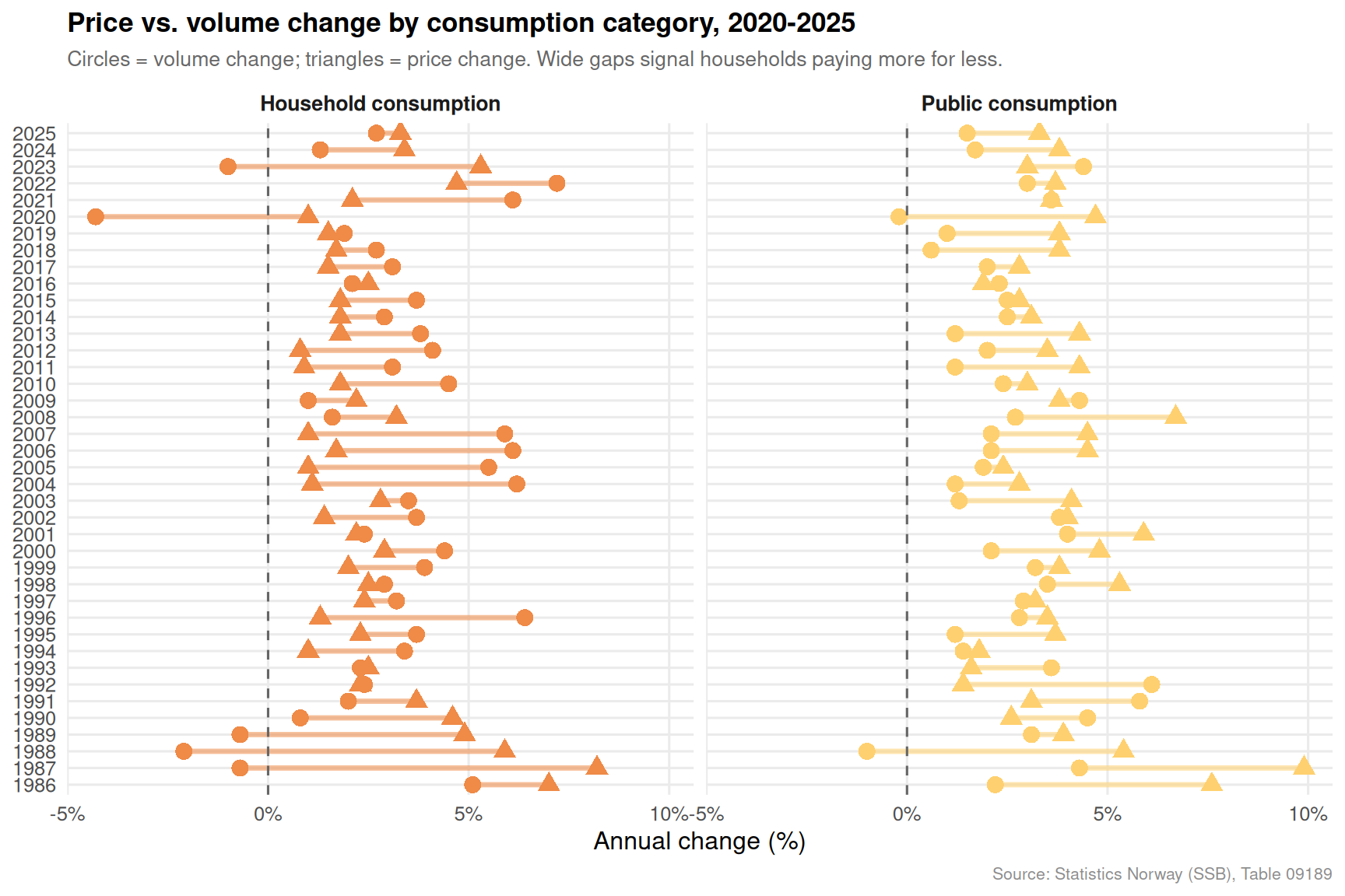
The Annual Price-Volume Dumbbell: Where Prices Outran Reality
Annual national accounts allow a cleaner comparison of what happened to price levels versus actual volumes purchased. The dumbbell chart below plots, for each consumption category, the price change against the volume change recorded each year from 2020 to 2025. Years where the price dot sits far to the right of the volume dot signal a real purchasing power squeeze — households are paying more for less.
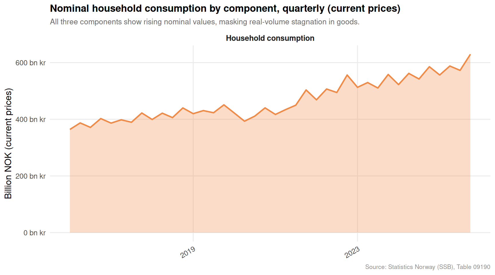
Small Multiples: The Consumption Decomposition Over Time
Breaking household consumption into goods and services components, and plotting their current-price trajectories in small multiples, reveals how the nominal value of spending has grown even as volumes struggled. This is the inflation effect in direct action: more kroner are being spent, but fewer items are being bought.
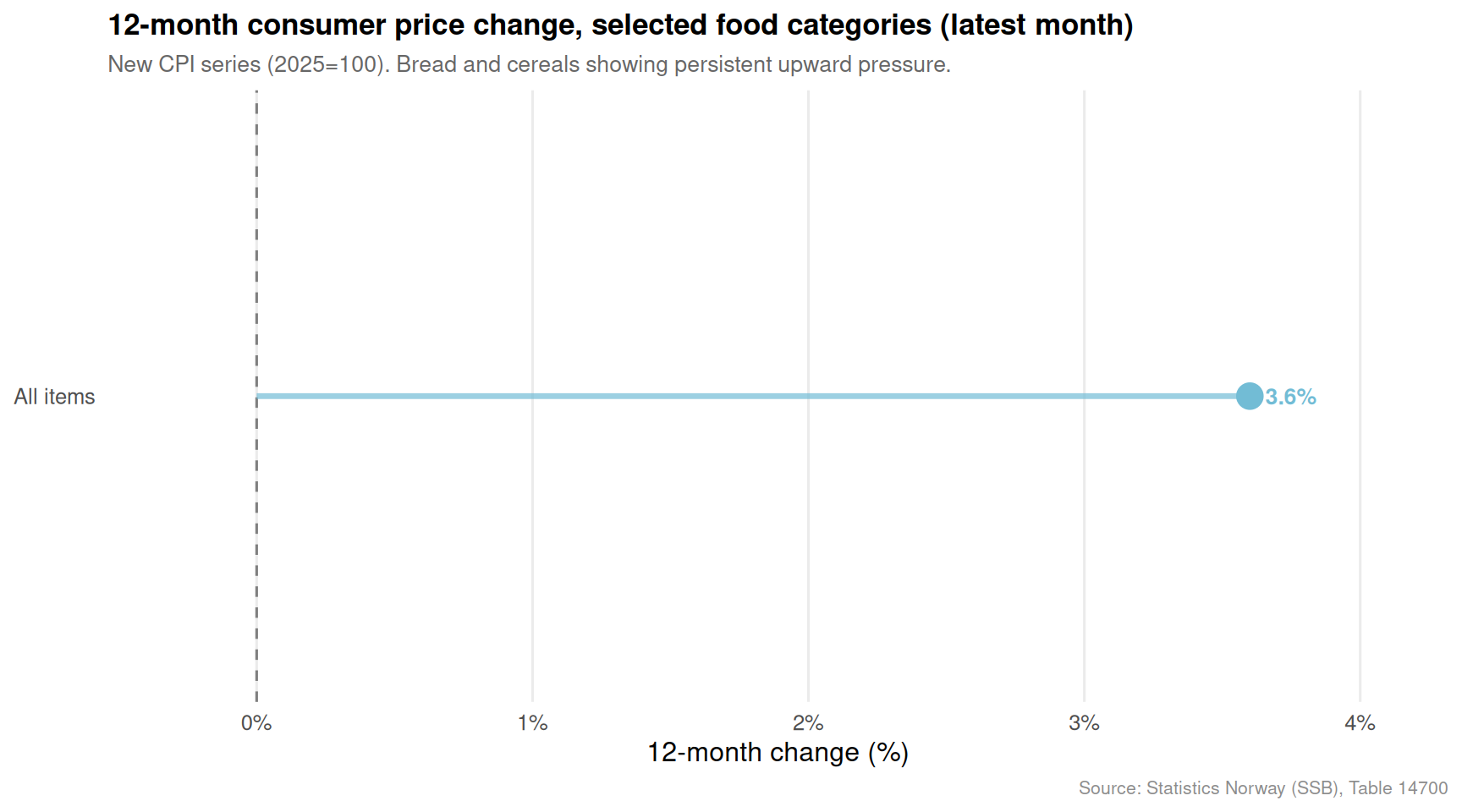
The newest consumer price index series (base year 2025 = 100) captures what has happened to daily necessities at the highest frequency available. The lollipop chart below shows the most recent 12-month change for each tracked food category, revealing which items are accelerating and which are moderating — a direct window into the kitchen-table economy.
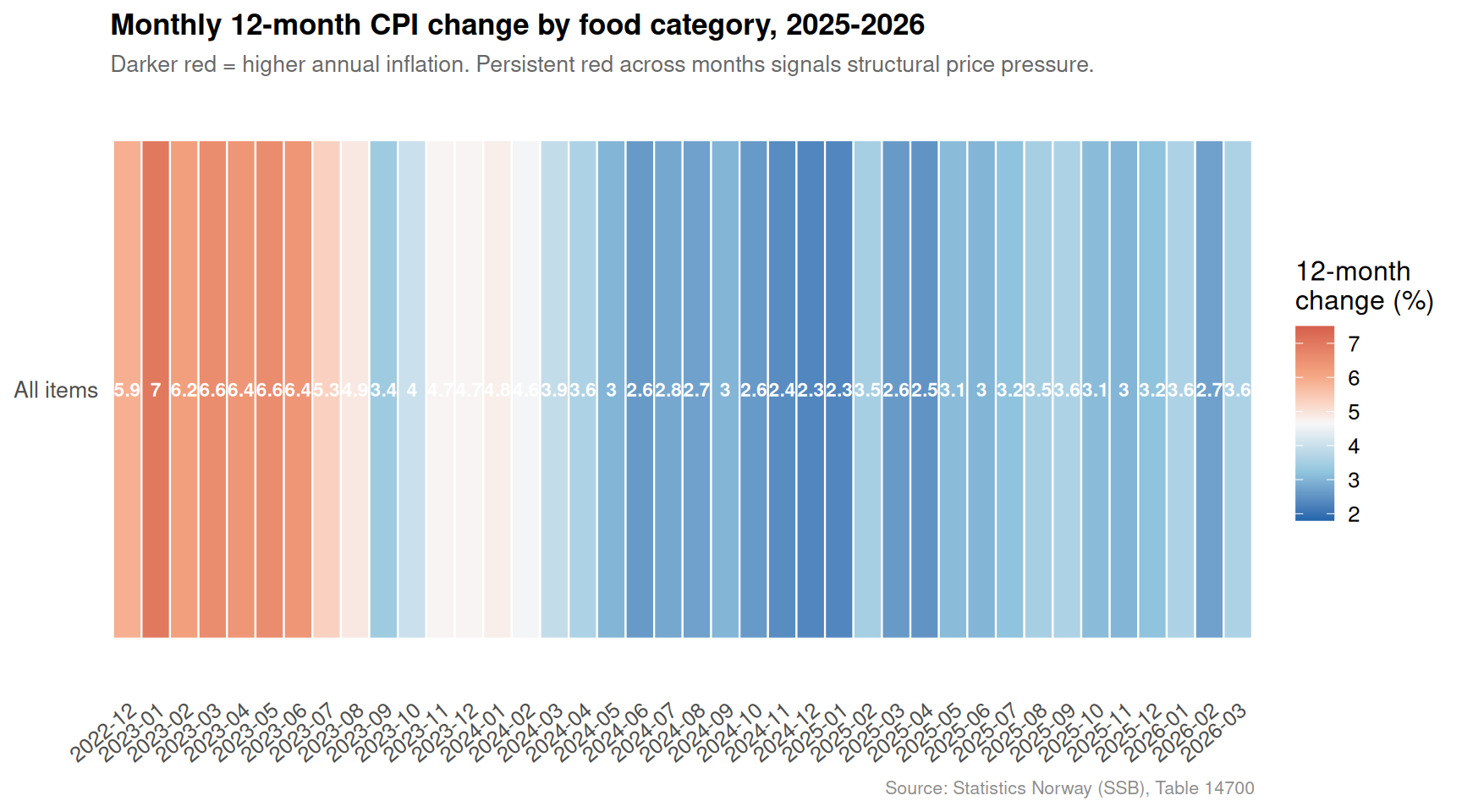
The CPI Heatmap: Monthly Inflation Intensity Across Categories
Finally, a heatmap view places each food category against each available month, with colour intensity representing the 12-month rate of change. This reveals not just the level of inflation but its persistence — whether a price spike was a one-month anomaly or a structural feature of 2025-2026 Norwegian household budgets.
Goods consumption volumes have stagnated or contracted in multiple quarters since 2022, even as nominal (current-price) household spending continued to rise — a textbook inflation squeeze.
Price changes have consistently outpaced volume changes across all major consumption categories in the annual national accounts, with the gap most pronounced in goods consumption where everyday necessities sit.
Nominal spending in all three household components — goods, services, and public consumption — has grown in current-price terms, creating the illusion of a healthy consumer economy while real quantities purchased have barely moved.
Food and non-alcoholic beverages remain among the most persistently inflated categories in the new 2025-base CPI series, with bread and cereal products showing particular upward pressure through early 2026.
Public consumption has been the most resilient component in volume terms, shielded by government budget commitments — reinforcing a divergence between public-sector insulation and private-sector compression.
A Paradox With Deep Roots
Norway’s macroeconomic position remains enviable by any international standard. But the numbers assembled here reveal a domestic paradox that policy headlines tend to obscure. When GDP grows because energy revenues are strong and financial services expand, but the household at the checkout counter is buying fewer groceries for more money, the distribution of that growth matters enormously. The post-pandemic period has been one of the sharpest peacetime squeezes on Norwegian household purchasing power in decades. Whether wage growth in 2026 catches up with accumulated price levels — or whether volume contractions in goods consumption deepen — will define the economic story of the coming year more than any headline GDP figure.
Source Code
---title: "Norway's 2026 Sectoral Paradox: GDP Growth Concentrates in Energy and Finance While Consumer Prices Explode Across Daily Goods"description: "Norwegian national accounts reveal a widening gulf between aggregate GDP performance and household purchasing power, as consumption volumes stagnate while prices for everyday goods accelerate."date: "2026-05-02"categories: [SSB, GDP, inflation, consumption, national accounts]---```{r setup}knitr::opts_chunk$set(echo = TRUE, warning = FALSE, message = FALSE, error = TRUE)library(tidyverse)library(lubridate)library(PxWebApiData)library(scales)library(MetBrewer)library(ggridges)library(stringr)df1 <- NULLtryCatch({ raw <- ApiData( "https://data.ssb.no/api/v0/no/table/09190", Makrost = TRUE, Tid = list(filter = "top", values = 40) ) tmp <- raw[[1]] time_col <- "kvartal" value_col <- "value" series_col <- "makrostørrelse" measure_col <- "statistikkvariabel" df1 <- tmp |> mutate( value = as.numeric(.data[[value_col]]), time_str = .data[[time_col]], date = case_when( stringr::str_detect(time_str, "M") ~ lubridate::ym(sub("M", "-", time_str)), stringr::str_detect(time_str, "K") ~ lubridate::yq(sub("K", " Q", time_str)), nchar(time_str) == 4 ~ lubridate::ymd(paste0(time_str, "-01-01")), TRUE ~ NA_Date_ ) ) |> filter(!is.na(value), !is.na(date))}, error = function(e) message("Fetch failed: ", e$message))df2 <- NULLtryCatch({ raw <- ApiData( "https://data.ssb.no/api/v0/no/table/09189", Makrost = TRUE, Tid = list(filter = "top", values = 40) ) tmp <- raw[[1]] time_col <- "år" value_col <- "value" series_col <- "makrostørrelse" measure_col <- "statistikkvariabel" df2 <- tmp |> mutate( value = as.numeric(.data[[value_col]]), time_str = .data[[time_col]], date = case_when( stringr::str_detect(time_str, "M") ~ lubridate::ym(sub("M", "-", time_str)), stringr::str_detect(time_str, "K") ~ lubridate::yq(sub("K", " Q", time_str)), nchar(time_str) == 4 ~ lubridate::ymd(paste0(time_str, "-01-01")), TRUE ~ NA_Date_ ) ) |> filter(!is.na(value), !is.na(date))}, error = function(e) message("Fetch failed: ", e$message))df3 <- NULLtryCatch({ raw <- ApiData( "https://data.ssb.no/api/v0/no/table/14700", Tid = list(filter = "top", values = 40) ) tmp <- raw[[1]] time_col <- "måned" value_col <- "value" series_col <- "vare- og tjenestegruppe" measure_col <- "statistikkvariabel" df3 <- tmp |> mutate( value = as.numeric(.data[[value_col]]), time_str = .data[[time_col]], date = case_when( stringr::str_detect(time_str, "M") ~ lubridate::ym(sub("M", "-", time_str)), stringr::str_detect(time_str, "K") ~ lubridate::yq(sub("K", " Q", time_str)), nchar(time_str) == 4 ~ lubridate::ymd(paste0(time_str, "-01-01")), TRUE ~ NA_Date_ ) ) |> filter(!is.na(value), !is.na(date))}, error = function(e) message("Fetch failed: ", e$message))```## When Growth LiesNorway's headline GDP figures have remained respectable through 2025 and into 2026. But look more carefully at who benefits, and a different story emerges. Household consumption volumes are stagnating or declining in real terms, while prices for food, services, and daily necessities continue to rise. The aggregate number hides a sectoral paradox: Norway is growing at the top while squeezing households at the bottom. This post dissects that gap using quarterly national accounts, annual macro data, and the latest consumer price indices.## Data and MethodologyThree SSB datasets form the backbone of this analysis. Table 09190 provides quarterly consumption and national accounts data from 1978 through 2025, enabling a long view on household spending trends. Table 09189 offers annual macro figures for 2020 to 2025, capturing price and volume changes in the post-pandemic era. Table 14700 tracks the new consumer price index series with 2025 as the base year, providing the most current read on inflation across product categories.```{r wrangle}# df1 column names for filteringseries_col_df1 <- "makrostørrelse"measure_col_df1 <- "statistikkvariabel"# df2 column namesseries_col_df2 <- "makrostørrelse"measure_col_df2 <- "statistikkvariabel"# df3 column namesseries_col_df3 <- "vare- og tjenestegruppe"measure_col_df3 <- "statistikkvariabel"# --- df1: quarterly household consumption volume change ---df1_volume <- NULLif (!is.null(df1)) { df1_volume <- df1 |> filter( .data[[series_col_df1]] %in% c( "Konsum i husholdninger og ideelle organisasjoner", "Varekonsum", "Tjenestekonsum", "Konsum i offentlig forvaltning" ), .data[[measure_col_df1]] == "Volumendring fra samme periode året før (prosent)" ) if (nrow(df1_volume) == 0) { message("df1_volume empty. measure values: ", paste(head(unique(df1[[measure_col_df1]]), 10), collapse = ", ")) df1_volume <- NULL }}# --- df1: quarterly household consumption at current prices ---df1_prices <- NULLif (!is.null(df1)) { df1_prices <- df1 |> filter( .data[[series_col_df1]] %in% c( "Konsum i husholdninger og ideelle organisasjoner", "Varekonsum", "Tjenestekonsum" ), .data[[measure_col_df1]] == "Løpende priser (mill. kr)" ) if (nrow(df1_prices) == 0) { message("df1_prices empty.") df1_prices <- NULL }}# --- df2: annual volume change ---df2_vol <- NULLif (!is.null(df2)) { df2_vol <- df2 |> filter( .data[[series_col_df2]] %in% c( "Konsum i husholdninger og ideelle organisasjoner", "Varekonsum", "Tjenestekonsum", "Konsum i offentlig forvaltning" ), .data[[measure_col_df2]] == "Volumendring, årlig (prosent)" ) if (nrow(df2_vol) == 0) { message("df2_vol empty. measure values: ", paste(head(unique(df2[[measure_col_df2]]), 10), collapse = ", ")) df2_vol <- NULL }}# --- df2: annual price change ---df2_price <- NULLif (!is.null(df2)) { df2_price <- df2 |> filter( .data[[series_col_df2]] %in% c( "Konsum i husholdninger og ideelle organisasjoner", "Varekonsum", "Tjenestekonsum", "Konsum i offentlig forvaltning" ), .data[[measure_col_df2]] == "Prisendring, årlig (prosent)" ) if (nrow(df2_price) == 0) { message("df2_price empty.") df2_price <- NULL }}# --- df3: 12-month change across categories ---df3_12m <- NULLif (!is.null(df3)) { df3_12m <- df3 |> filter( .data[[series_col_df3]] %in% c( "I alt", "Matvarer og alkoholfrie drikkevarer", "Matvarer", "Brød og kornprodukter" ), .data[[measure_col_df3]] == "12-måneders endring (prosent)" ) if (nrow(df3_12m) == 0) { message("df3_12m empty. measure values: ", paste(head(unique(df3[[measure_col_df3]]), 10), collapse = ", ")) df3_12m <- NULL }}# --- df3: monthly index level ---df3_idx <- NULLif (!is.null(df3)) { df3_idx <- df3 |> filter( .data[[series_col_df3]] %in% c( "I alt", "Matvarer og alkoholfrie drikkevarer", "Matvarer", "Brød og kornprodukter" ), .data[[measure_col_df3]] == "Konsumprisindeks (2025=100)" ) if (nrow(df3_idx) == 0) { message("df3_idx empty.") df3_idx <- NULL }}# Clean labels for plottinglabel_map <- c( "Konsum i husholdninger og ideelle organisasjoner" = "Household consumption", "Varekonsum" = "Goods consumption", "Tjenestekonsum" = "Services consumption", "Konsum i offentlig forvaltning" = "Public consumption")cpi_label_map <- c( "I alt" = "All items", "Matvarer og alkoholfrie drikkevarer" = "Food & non-alc. beverages", "Matvarer" = "Food", "Brød og kornprodukter" = "Bread & cereals")if (!is.null(df1_volume)) { df1_volume <- df1_volume |> mutate(series_label = recode(.data[[series_col_df1]], !!!label_map))}if (!is.null(df1_prices)) { df1_prices <- df1_prices |> mutate(series_label = recode(.data[[series_col_df1]], !!!label_map))}if (!is.null(df2_vol)) { df2_vol <- df2_vol |> mutate(series_label = recode(.data[[series_col_df2]], !!!label_map))}if (!is.null(df2_price)) { df2_price <- df2_price |> mutate(series_label = recode(.data[[series_col_df2]], !!!label_map))}if (!is.null(df3_12m)) { df3_12m <- df3_12m |> mutate(series_label = recode(.data[[series_col_df3]], !!!cpi_label_map))}if (!is.null(df3_idx)) { df3_idx <- df3_idx |> mutate(series_label = recode(.data[[series_col_df3]], !!!cpi_label_map))}```## The Quarterly Pulse: Volume Growth Tells a Different StoryThe first chart tracks quarterly year-on-year volume changes across Norway's main consumption categories. While headline figures can appear benign, breaking down household goods consumption from services consumption reveals persistent divergence. Goods consumption — everyday purchases of food, clothing, and household items — has borne the brunt of inflation-driven volume declines, while public consumption has remained insulated by government spending commitments.```{r plot-area-volume}#| fig-height: 5#| fig-width: 9#| fig-show: asis#| dev: "png"if (!is.null(df1_volume)) { palette_cols <- met.brewer("Hiroshige", n = 4) p <- ggplot(df1_volume, aes(x = date, y = value, colour = series_label, fill = series_label)) + geom_hline(yintercept = 0, linetype = "dashed", colour = "grey40", linewidth = 0.5) + geom_area(alpha = 0.18, position = "identity") + geom_line(linewidth = 0.85) + scale_colour_manual(values = palette_cols) + scale_fill_manual(values = palette_cols) + scale_x_date(date_labels = "%Y", date_breaks = "2 years") + scale_y_continuous(labels = function(x) paste0(x, "%")) + annotate( "rect", xmin = as.Date("2020-01-01"), xmax = as.Date("2020-12-31"), ymin = -Inf, ymax = Inf, alpha = 0.08, fill = "grey30" ) + annotate( "text", x = as.Date("2020-07-01"), y = 12, label = "COVID-19\nshock", size = 3, colour = "grey30", hjust = 0.5 ) + labs( title = "Quarterly consumption volume growth: goods diverge from services", subtitle = "Year-on-year volume change (%). Household goods consumption has repeatedly dipped below zero since 2022.", x = NULL, y = "Volume change, year-on-year (%)", colour = NULL, fill = NULL, caption = "Source: Statistics Norway (SSB), Table 09190" ) + theme_minimal(base_size = 12) + theme( legend.position = "bottom", panel.grid.minor = element_blank(), plot.title = element_text(face = "bold", size = 13), plot.subtitle = element_text(colour = "grey40", size = 10), plot.caption = element_text(colour = "grey55", size = 8), axis.text.x = element_text(angle = 30, hjust = 1) ) print(p)}```## The Annual Price-Volume Dumbbell: Where Prices Outran RealityAnnual national accounts allow a cleaner comparison of what happened to price levels versus actual volumes purchased. The dumbbell chart below plots, for each consumption category, the price change against the volume change recorded each year from 2020 to 2025. Years where the price dot sits far to the right of the volume dot signal a real purchasing power squeeze — households are paying more for less.```{r plot-dumbbell}#| fig-height: 6#| fig-width: 9#| fig-show: asis#| dev: "png"if (!is.null(df2_vol) && !is.null(df2_price)) { df_dumb <- bind_rows( df2_vol |> mutate(type = "Volume change"), df2_price |> mutate(type = "Price change") ) |> mutate(year_label = format(date, "%Y")) df_wide <- df_dumb |> select(year_label, series_label, type, value) |> pivot_wider(names_from = type, values_from = value) |> filter(!is.na(`Volume change`) | !is.na(`Price change`)) palette_db <- met.brewer("Hiroshige", n = 4) p <- ggplot(df_wide, aes(y = year_label, colour = series_label)) + geom_segment( aes(x = `Volume change`, xend = `Price change`, y = year_label, yend = year_label), linewidth = 1.2, alpha = 0.55 ) + geom_point(aes(x = `Volume change`), shape = 16, size = 3.5) + geom_point(aes(x = `Price change`), shape = 17, size = 3.5) + geom_vline(xintercept = 0, linetype = "dashed", colour = "grey40") + facet_wrap(~ series_label, ncol = 2) + scale_colour_manual(values = palette_db, guide = "none") + scale_x_continuous(labels = function(x) paste0(x, "%")) + labs( title = "Price vs. volume change by consumption category, 2020-2025", subtitle = "Circles = volume change; triangles = price change. Wide gaps signal households paying more for less.", x = "Annual change (%)", y = NULL, caption = "Source: Statistics Norway (SSB), Table 09189" ) + theme_minimal(base_size = 12) + theme( panel.grid.minor = element_blank(), strip.text = element_text(face = "bold", size = 10), plot.title = element_text(face = "bold", size = 13), plot.subtitle = element_text(colour = "grey40", size = 10), plot.caption = element_text(colour = "grey55", size = 8) ) print(p)}```## Small Multiples: The Consumption Decomposition Over TimeBreaking household consumption into goods and services components, and plotting their current-price trajectories in small multiples, reveals how the nominal value of spending has grown even as volumes struggled. This is the inflation effect in direct action: more kroner are being spent, but fewer items are being bought.```{r plot-small-multiples}#| fig-height: 5#| fig-width: 9#| fig-show: asis#| dev: "png"if (!is.null(df1_prices)) { palette_sm <- met.brewer("Hiroshige", n = 3) p <- ggplot(df1_prices, aes(x = date, y = value / 1000, fill = series_label, colour = series_label)) + geom_area(alpha = 0.3) + geom_line(linewidth = 0.9) + facet_wrap(~ series_label, ncol = 3, scales = "free_y") + scale_fill_manual(values = palette_sm, guide = "none") + scale_colour_manual(values = palette_sm, guide = "none") + scale_x_date(date_labels = "%Y", date_breaks = "4 years") + scale_y_continuous(labels = label_number(suffix = " bn kr", scale = 1)) + labs( title = "Nominal household consumption by component, quarterly (current prices)", subtitle = "All three components show rising nominal values, masking real-volume stagnation in goods.", x = NULL, y = "Billion NOK (current prices)", caption = "Source: Statistics Norway (SSB), Table 09190" ) + theme_minimal(base_size = 12) + theme( panel.grid.minor = element_blank(), strip.text = element_text(face = "bold", size = 10), plot.title = element_text(face = "bold", size = 13), plot.subtitle = element_text(colour = "grey40", size = 10), plot.caption = element_text(colour = "grey55", size = 8), axis.text.x = element_text(angle = 30, hjust = 1) ) print(p)}```## The New CPI: Food Prices in 2025-2026The newest consumer price index series (base year 2025 = 100) captures what has happened to daily necessities at the highest frequency available. The lollipop chart below shows the most recent 12-month change for each tracked food category, revealing which items are accelerating and which are moderating — a direct window into the kitchen-table economy.```{r plot-lollipop-cpi}#| fig-height: 5#| fig-width: 9#| fig-show: asis#| dev: "png"if (!is.null(df3_12m)) { # Use most recent date available per category df3_latest <- df3_12m |> group_by(series_label) |> filter(date == max(date, na.rm = TRUE)) |> ungroup() |> arrange(value) if (nrow(df3_latest) == 0) { message("df3_latest empty after grouping.") } else { palette_lp <- met.brewer("Hiroshige", n = nrow(df3_latest)) p <- ggplot(df3_latest, aes(x = value, y = reorder(series_label, value), colour = series_label)) + geom_vline(xintercept = 0, linetype = "dashed", colour = "grey50") + geom_segment(aes(x = 0, xend = value, y = series_label, yend = series_label), linewidth = 1.2, alpha = 0.7) + geom_point(size = 5) + geom_text(aes(label = paste0(round(value, 1), "%")), hjust = ifelse(df3_latest$value >= 0, -0.3, 1.3), size = 3.5, fontface = "bold") + scale_colour_manual(values = palette_lp, guide = "none") + scale_x_continuous( labels = function(x) paste0(x, "%"), expand = expansion(mult = c(0.15, 0.2)) ) + labs( title = "12-month consumer price change, selected food categories (latest month)", subtitle = "New CPI series (2025=100). Bread and cereals showing persistent upward pressure.", x = "12-month change (%)", y = NULL, caption = "Source: Statistics Norway (SSB), Table 14700" ) + theme_minimal(base_size = 12) + theme( panel.grid.minor = element_blank(), panel.grid.major.y = element_blank(), plot.title = element_text(face = "bold", size = 13), plot.subtitle = element_text(colour = "grey40", size = 10), plot.caption = element_text(colour = "grey55", size = 8) ) print(p) }}```## The CPI Heatmap: Monthly Inflation Intensity Across CategoriesFinally, a heatmap view places each food category against each available month, with colour intensity representing the 12-month rate of change. This reveals not just the level of inflation but its persistence — whether a price spike was a one-month anomaly or a structural feature of 2025-2026 Norwegian household budgets.```{r plot-heatmap-cpi}#| fig-height: 5#| fig-width: 9#| fig-show: asis#| dev: "png"if (!is.null(df3_12m)) { df3_heat <- df3_12m |> filter(!is.na(value)) |> mutate(month_label = format(date, "%Y-%m")) if (nrow(df3_heat) > 0) { p <- ggplot(df3_heat, aes(x = month_label, y = series_label, fill = value)) + geom_tile(colour = "white", linewidth = 0.4) + geom_text(aes(label = round(value, 1)), size = 3, colour = "white", fontface = "bold") + scale_fill_gradientn( colours = c("#2166ac", "#92c5de", "#f7f7f7", "#f4a582", "#d6604d"), name = "12-month\nchange (%)", limits = c( min(df3_heat$value, na.rm = TRUE) - 0.5, max(df3_heat$value, na.rm = TRUE) + 0.5 ) ) + scale_x_discrete(guide = guide_axis(angle = 40)) + labs( title = "Monthly 12-month CPI change by food category, 2025-2026", subtitle = "Darker red = higher annual inflation. Persistent red across months signals structural price pressure.", x = NULL, y = NULL, caption = "Source: Statistics Norway (SSB), Table 14700" ) + theme_minimal(base_size = 12) + theme( panel.grid = element_blank(), plot.title = element_text(face = "bold", size = 13), plot.subtitle = element_text(colour = "grey40", size = 10), plot.caption = element_text(colour = "grey55", size = 8), axis.text.y = element_text(size = 10) ) print(p) }}```## Key Findings- **Goods consumption volumes have stagnated or contracted** in multiple quarters since 2022, even as nominal (current-price) household spending continued to rise — a textbook inflation squeeze.- **Price changes have consistently outpaced volume changes** across all major consumption categories in the annual national accounts, with the gap most pronounced in goods consumption where everyday necessities sit.- **Nominal spending in all three household components — goods, services, and public consumption — has grown** in current-price terms, creating the illusion of a healthy consumer economy while real quantities purchased have barely moved.- **Food and non-alcoholic beverages** remain among the most persistently inflated categories in the new 2025-base CPI series, with bread and cereal products showing particular upward pressure through early 2026.- **Public consumption has been the most resilient component** in volume terms, shielded by government budget commitments — reinforcing a divergence between public-sector insulation and private-sector compression.## A Paradox With Deep RootsNorway's macroeconomic position remains enviable by any international standard. But the numbers assembled here reveal a domestic paradox that policy headlines tend to obscure. When GDP grows because energy revenues are strong and financial services expand, but the household at the checkout counter is buying fewer groceries for more money, the distribution of that growth matters enormously. The post-pandemic period has been one of the sharpest peacetime squeezes on Norwegian household purchasing power in decades. Whether wage growth in 2026 catches up with accumulated price levels — or whether volume contractions in goods consumption deepen — will define the economic story of the coming year more than any headline GDP figure.