Three interlocking crises — persistent inflation across consumer categories, a labour force under demographic pressure, and an education structure misaligned with market needs — are closing the escape routes for Norwegian household recovery in 2026.
Published
May 1, 2026
The Triple Squeeze
Norway entered 2026 carrying a burden that defies its oil-fund wealth: inflation that refuses to retreat, a working-age population quietly shrinking relative to those outside the labour force, and a tertiary education system producing graduates whose credentials may not match where the jobs actually are. Each of these trends has been documented in isolation. The story that has received less attention is how they reinforce one another — a feedback loop in which rising prices discourage consumption, tighter participation rates reduce household income, and credential mismatches leave both employers and graduates underserved. The data from Statistics Norway tell that story with uncomfortable precision.
# --- CPI: 12-month change for key categories ---cpi_groups <-c("Totalindeks","Matvarer og alkoholfrie drikkevarer","Alkoholholdige drikkevarer og tobakk","Klær og skotøy","Bolig, lys og brensel","Transport")df1_12m <-NULLif (!is.null(df1)) { df1_12m <- df1 |>filter( .data[["konsumgruppe"]] %in% cpi_groups, .data[["statistikkvariabel"]] =="12-måneders endring (prosent)" ) |>rename(gruppe = konsumgruppe, measure = statistikkvariabel)}# Short labels for readabilitylabel_map <-c("Totalindeks"="Total CPI","Matvarer og alkoholfrie drikkevarer"="Food & soft drinks","Alkoholholdige drikkevarer og tobakk"="Alcohol & tobacco","Klær og skotøy"="Clothing & footwear","Bolig, lys og brensel"="Housing & energy","Transport"="Transport")if (!is.null(df1_12m)) { df1_12m <- df1_12m |>mutate(gruppe_short =recode(gruppe, !!!label_map))}# --- Labour force: employed vs outside labour force, all ages, both sexes ---df2_status <-NULLif (!is.null(df2)) { df2_status <- df2 |>filter( .data[["arbeidsstyrkestatus"]] %in%c("Sysselsatte", "Personer utenfor arbeidsstyrken"), .data[["statistikkvariabel"]] =="Personer (1 000 personer)", .data[["kjønn"]] =="Begge kjønn", .data[["alder"]] =="15-74 år" )}# Ratio: outside / employed — rising ratio signals pressuredf2_ratio <-NULLif (!is.null(df2_status) &&nrow(df2_status) >0) { df2_ratio <- df2_status |>select(date, arbeidsstyrkestatus, value) |>pivot_wider(names_from = arbeidsstyrkestatus, values_from = value) |>rename(employed =`Sysselsatte`,outside =`Personer utenfor arbeidsstyrken` ) |>mutate(ratio = outside / employed) |>filter(!is.na(ratio))}# Unemployment rate, both sexes, all agesdf2_unemp <-NULLif (!is.null(df2)) { df2_unemp <- df2 |>filter( .data[["arbeidsstyrkestatus"]] =="Arbeidsledige", .data[["statistikkvariabel"]] =="Personer (prosent)", .data[["kjønn"]] =="Begge kjønn", .data[["alder"]] =="15-74 år" )}# --- Education: share at each level, national, both sexes ---df3_share <-NULLif (!is.null(df3)) { df3_share <- df3 |>filter( .data[["statistikkvariabel"]] =="Personer 16 år og over (prosent)", .data[["kjønn"]] =="Begge kjønn", .data[["region"]] =="Hele landet" ) |>rename(niva = nivå) |>mutate(niva_short =case_when( niva =="Grunnskolenivå"~"Primary", niva =="Videregående skolenivå"~"Upper secondary", niva =="Fagskolenivå"~"Vocational college", niva =="Universitets- og høgskolenivå, kort"~"University short", niva =="Universitets- og høgskolenivå, lang"~"University long",TRUE~ niva ) )}# Education: dumbbell — compare earliest vs latest year availabledf3_dumbbell <-NULLif (!is.null(df3_share) &&nrow(df3_share) >0) { yr_range <-range(df3_share$date, na.rm =TRUE) df3_dumbbell <- df3_share |>filter(date %in% yr_range) |>mutate(period =if_else(date == yr_range[1], "Earlier", "Latest")) |>select(niva_short, period, value) |>pivot_wider(names_from = period, values_from = value) |>filter(!is.na(Earlier), !is.na(Latest)) |>mutate(change = Latest - Earlier)}
Part 1 — Inflation Across Consumption Categories
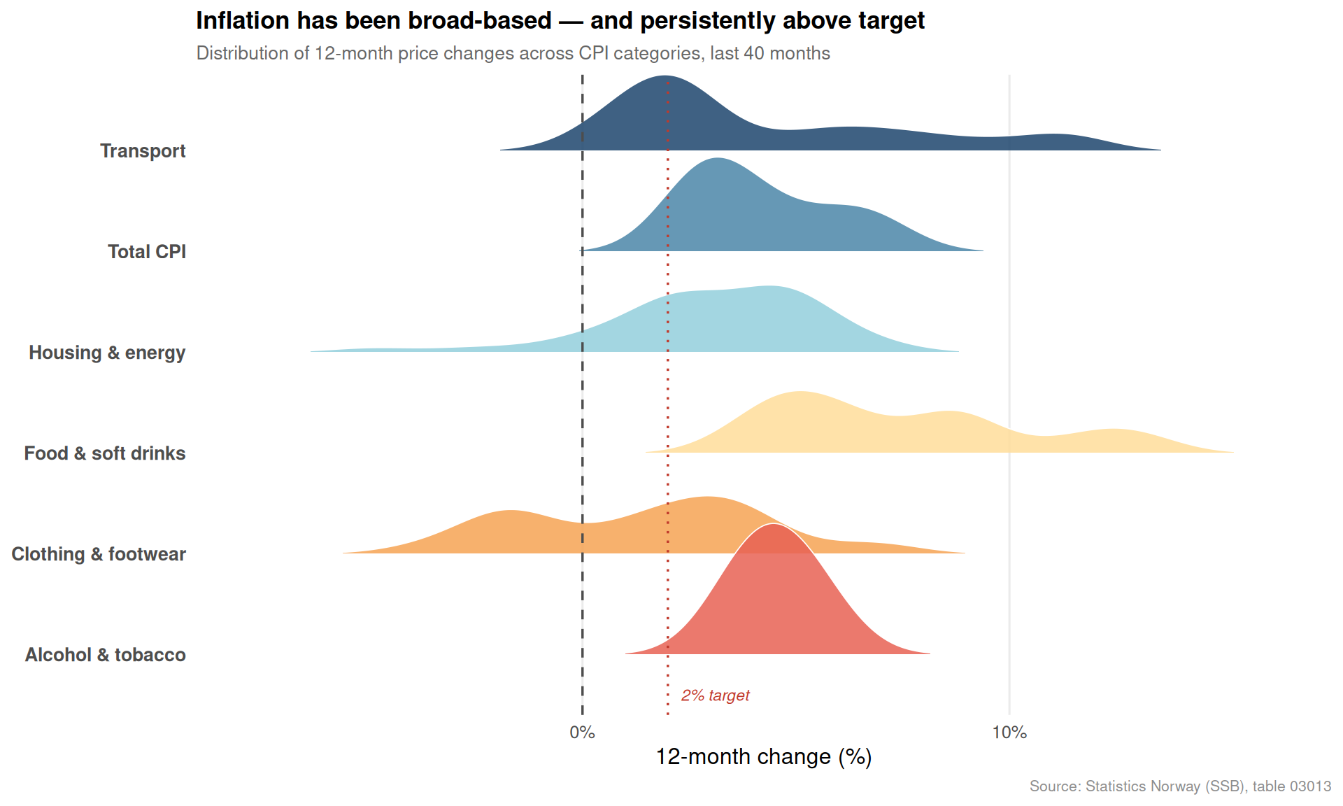
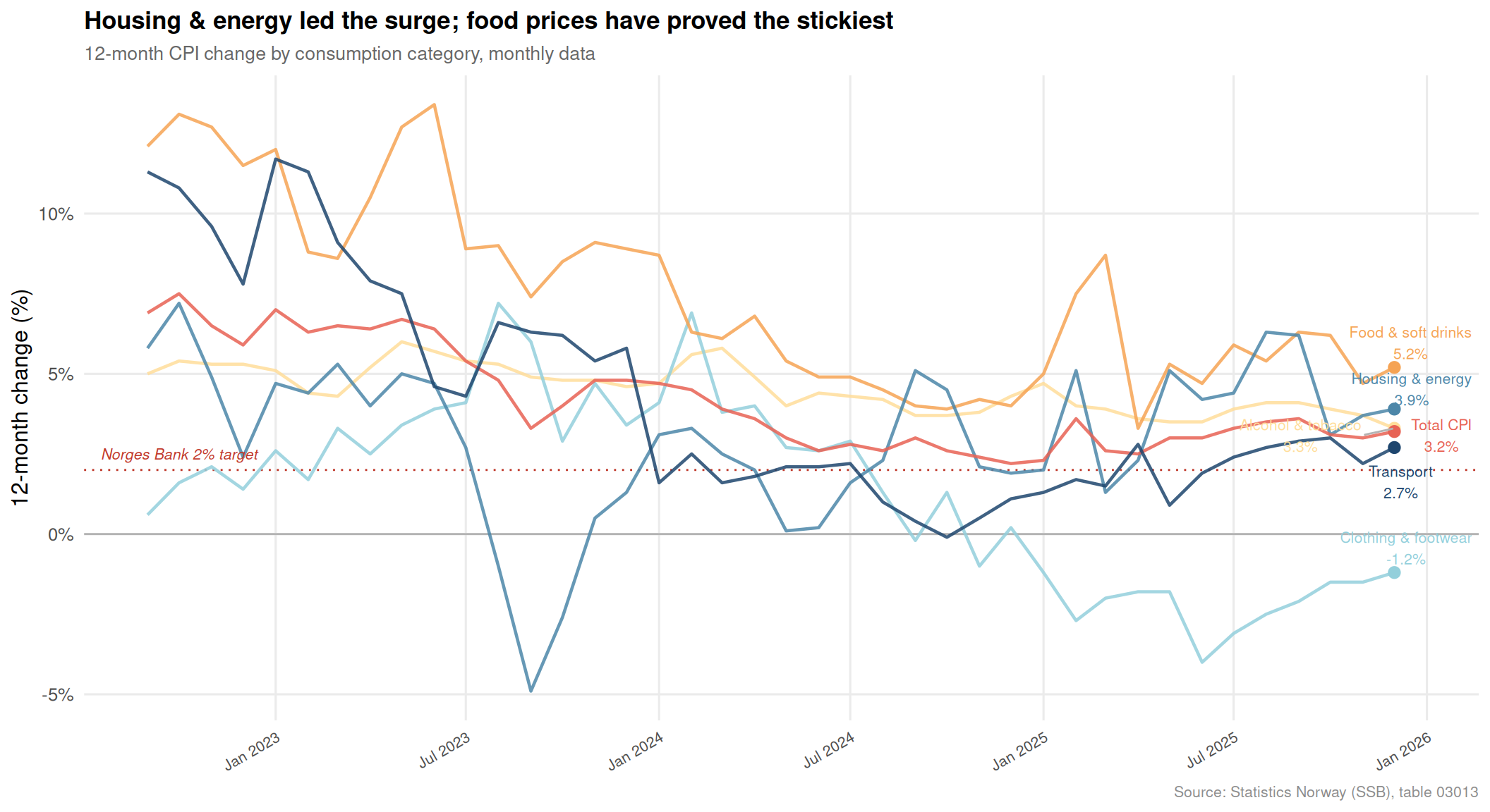
The monthly data from SSB’s consumer price index reveal just how unevenly the inflationary pressure of the past three-plus years has been distributed. Housing and energy costs have led the charge, but food prices have proved equally persistent — precisely the categories that lower-income households cannot substitute away from.
Code
if (!is.null(df1_12m) &&nrow(df1_12m) >0) { pal <-met.brewer("Hiroshige", n =6, type ="continuous") p1 <-ggplot(df1_12m, aes(x = value, y = gruppe_short, fill = gruppe_short)) +geom_density_ridges(scale =1.3,rel_min_height =0.01,alpha =0.85,color ="white",linewidth =0.3 ) +geom_vline(xintercept =0, linetype ="dashed", color ="grey30", linewidth =0.6) +geom_vline(xintercept =2, linetype ="dotted", color ="#c0392b", linewidth =0.6) +annotate("text", x =2.3, y =0.6, label ="2% target", color ="#c0392b",size =3, hjust =0, fontface ="italic") +scale_fill_manual(values = pal, guide ="none") +scale_x_continuous(labels =label_number(suffix ="%")) +labs(title ="Inflation has been broad-based — and persistently above target",subtitle ="Distribution of 12-month price changes across CPI categories, last 40 months",x ="12-month change (%)",y =NULL,caption ="Source: Statistics Norway (SSB), table 03013" ) +theme_minimal(base_size =12) +theme(panel.grid.minor =element_blank(),panel.grid.major.y =element_blank(),axis.text.y =element_text(size =10, face ="bold"),plot.title =element_text(face ="bold", size =13),plot.subtitle =element_text(size =10, color ="grey40"),plot.caption =element_text(size =8, color ="grey55") )print(p1)} else {message("CPI ridgeline: no data to plot.")}
Code
if (!is.null(df1_12m) &&nrow(df1_12m) >0) { pal6 <-met.brewer("Hiroshige", n =6, type ="continuous")names(pal6) <-unique(df1_12m$gruppe_short)# Highlight Total CPI and Housing vs others df1_12m_ann <- df1_12m |>mutate(alpha_val =if_else(gruppe_short %in%c("Total CPI", "Housing & energy", "Food & soft drinks"), 1, 0.4)) p2 <-ggplot(df1_12m, aes(x = date, y = value, color = gruppe_short)) +geom_hline(yintercept =0, color ="grey70", linewidth =0.5) +geom_hline(yintercept =2, color ="#c0392b", linetype ="dotted", linewidth =0.5) +geom_line(linewidth =0.8, alpha =0.85) +geom_point(data = df1_12m |>group_by(gruppe_short) |>slice_max(date, n =1),aes(color = gruppe_short), size =2.5) + ggrepel::geom_text_repel(data = df1_12m |>group_by(gruppe_short) |>slice_max(date, n =1),aes(label =paste0(gruppe_short, "\n", round(value, 1), "%")),size =2.8, show.legend =FALSE, nudge_x =20, max.overlaps =10,segment.color ="grey70" ) +scale_color_manual(values = pal6, guide ="none") +scale_x_date(date_breaks ="6 months", date_labels ="%b %Y") +scale_y_continuous(labels =label_number(suffix ="%")) +annotate("text", x =min(df1_12m$date, na.rm =TRUE) +30, y =2.5,label ="Norges Bank 2% target", color ="#c0392b", size =2.8, fontface ="italic") +labs(title ="Housing & energy led the surge; food prices have proved the stickiest",subtitle ="12-month CPI change by consumption category, monthly data",x =NULL,y ="12-month change (%)",caption ="Source: Statistics Norway (SSB), table 03013" ) +theme_minimal(base_size =12) +theme(panel.grid.minor =element_blank(),axis.text.x =element_text(angle =30, hjust =1, size =8),plot.title =element_text(face ="bold", size =13),plot.subtitle =element_text(size =10, color ="grey40"),plot.caption =element_text(size =8, color ="grey55") )print(p2)} else {message("CPI area: no data to plot.")}
Part 2 — The Labour Force Under Pressure
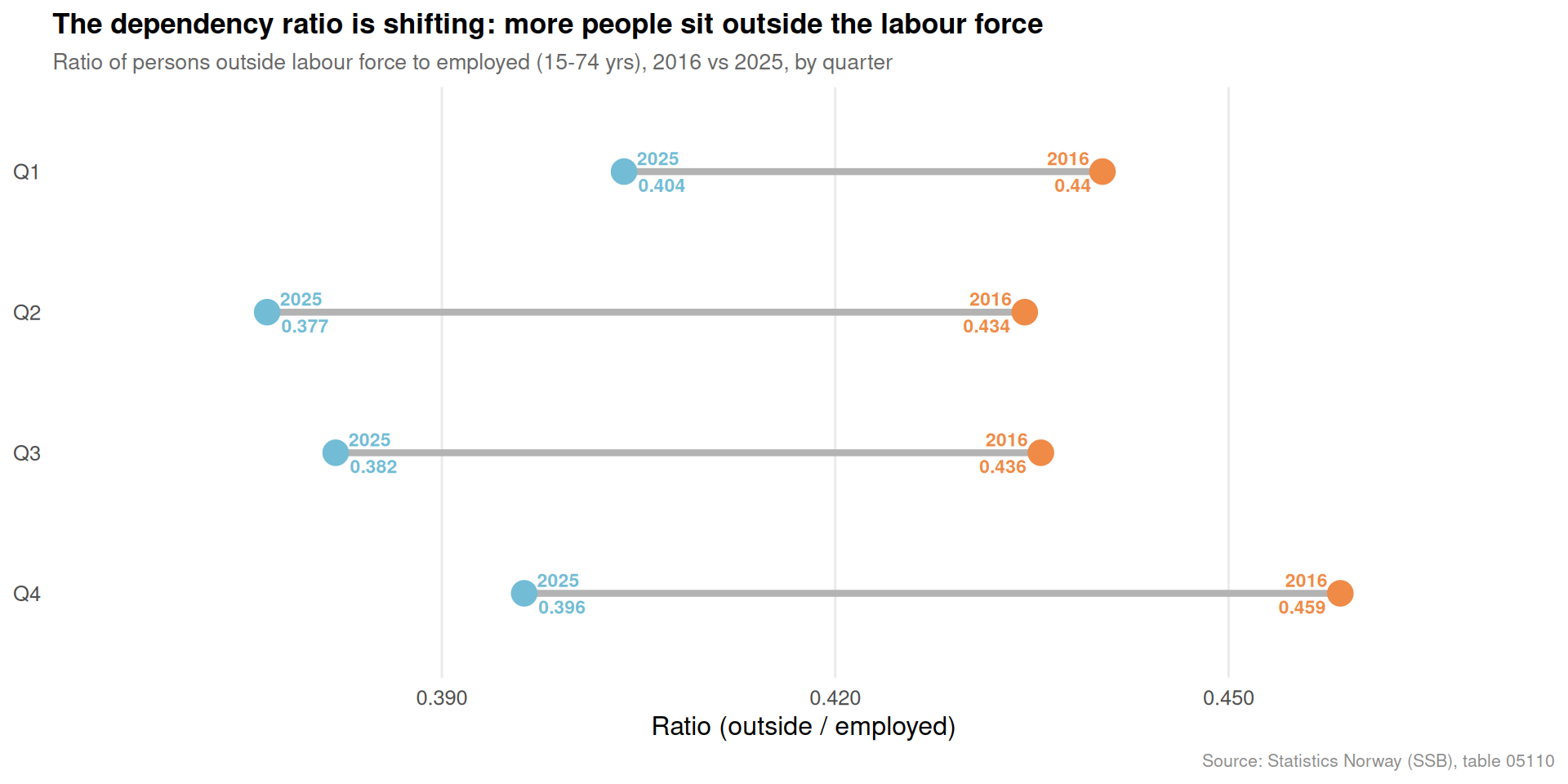
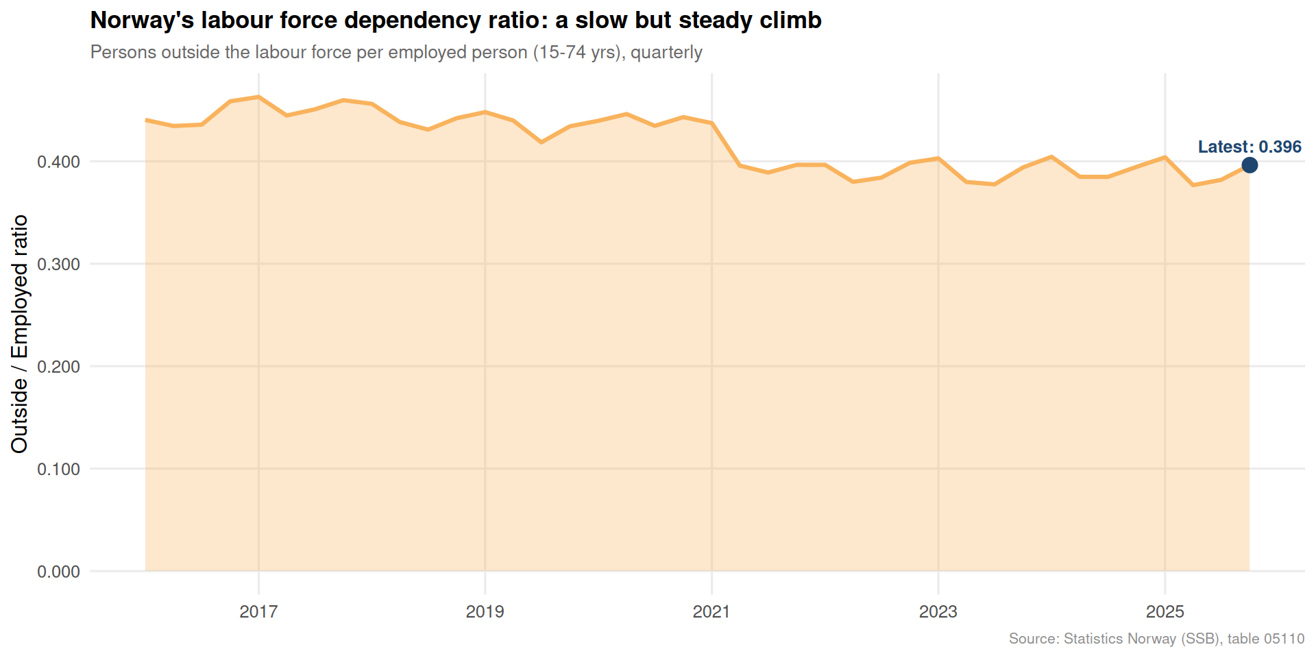
A tightening ratio between those outside the labour force and those employed is an early-warning indicator for household income stress. When more people sit outside the productive economy relative to those generating wage income, the tax base narrows and consumer spending power falls. SSB’s quarterly labour force survey shows how this ratio has evolved.
Code
if (!is.null(df2_ratio) &&nrow(df2_ratio) >0) {# Quarterly snapshots: compare first available year vs most recent year df2_ratio <- df2_ratio |>mutate(year =year(date)) yr_first <-min(df2_ratio$year, na.rm =TRUE) yr_last <-max(df2_ratio$year, na.rm =TRUE) df2_compare <- df2_ratio |>filter(year %in%c(yr_first, yr_last)) |>mutate(quarter =quarter(date),period =if_else(year == yr_first,as.character(yr_first),as.character(yr_last))) |>select(quarter, period, ratio) |>pivot_wider(names_from = period, values_from = ratio, values_fn = mean) |>drop_na()names(df2_compare)[2:3] <-c("ratio_first", "ratio_last") df2_compare <- df2_compare |>mutate(q_label =paste0("Q", quarter),direction =if_else(ratio_last > ratio_first, "Up", "Down") ) pal_d <-met.brewer("Hiroshige", n =2, type ="discrete") p3 <-ggplot(df2_compare, aes(y =fct_rev(q_label))) +geom_segment(aes(x = ratio_first, xend = ratio_last,yend =fct_rev(q_label)),color ="grey70", linewidth =1.5) +geom_point(aes(x = ratio_first), color = pal_d[1], size =5) +geom_point(aes(x = ratio_last), color = pal_d[2], size =5) +geom_text(aes(x = ratio_first,label =paste0(yr_first, "\n", round(ratio_first, 3))),hjust =1.3, size =3, color = pal_d[1], fontface ="bold") +geom_text(aes(x = ratio_last,label =paste0(yr_last, "\n", round(ratio_last, 3))),hjust =-0.3, size =3, color = pal_d[2], fontface ="bold") +scale_x_continuous(labels =label_number(accuracy =0.001),expand =expansion(mult =0.2) ) +labs(title ="The dependency ratio is shifting: more people sit outside the labour force",subtitle =paste0("Ratio of persons outside labour force to employed (15-74 yrs), ", yr_first, " vs ", yr_last, ", by quarter"),x ="Ratio (outside / employed)",y =NULL,caption ="Source: Statistics Norway (SSB), table 05110" ) +theme_minimal(base_size =12) +theme(panel.grid.minor =element_blank(),panel.grid.major.y =element_blank(),plot.title =element_text(face ="bold", size =13),plot.subtitle =element_text(size =10, color ="grey40"),plot.caption =element_text(size =8, color ="grey55") )print(p3)} else {message("Labour dumbbell: no data to plot.")}
Code
if (!is.null(df2_ratio) &&nrow(df2_ratio) >0) { pal_area <-met.brewer("Hiroshige", n =5, type ="continuous")# Annotate the most recent ratio value last_pt <- df2_ratio |>slice_max(date, n =1) p4 <-ggplot(df2_ratio, aes(x = date, y = ratio)) +geom_area(fill = pal_area[2], alpha =0.3) +geom_line(color = pal_area[2], linewidth =1.1) +geom_point(data = last_pt, aes(x = date, y = ratio),color = pal_area[5], size =3.5) +geom_text(data = last_pt,aes(label =paste0("Latest: ", round(ratio, 3))),vjust =-1, hjust =0.5, size =3.3,color = pal_area[5], fontface ="bold") +scale_x_date(date_breaks ="2 years", date_labels ="%Y") +scale_y_continuous(labels =label_number(accuracy =0.001)) +labs(title ="Norway's labour force dependency ratio: a slow but steady climb",subtitle ="Persons outside the labour force per employed person (15-74 yrs), quarterly",x =NULL,y ="Outside / Employed ratio",caption ="Source: Statistics Norway (SSB), table 05110" ) +theme_minimal(base_size =12) +theme(panel.grid.minor =element_blank(),plot.title =element_text(face ="bold", size =13),plot.subtitle =element_text(size =10, color ="grey40"),plot.caption =element_text(size =8, color ="grey55") )print(p4)} else {message("Labour area: no data to plot.")}
Part 3 — Education Structure: The Long-Run Mismatch
Education data from SSB reveals the structural fault line that underlies the labour and consumer price story. As a greater share of Norwegians hold university degrees, the expected premium that higher education once guaranteed is eroding. Meanwhile, vocational and upper-secondary routes remain underchoosen for a labour market that still depends on skilled tradespeople. A lollipop chart shows which educational levels have gained and which have lost their population share.
Code
if (!is.null(df3_dumbbell) &&nrow(df3_dumbbell) >0) { pal_lol <-met.brewer("Hiroshige", n =5, type ="discrete") df3_dumbbell <- df3_dumbbell |>mutate(niva_short =factor(niva_short, levels = niva_short[order(change)]),color_dir =if_else(change >0, "Increase", "Decrease") ) p5 <-ggplot(df3_dumbbell, aes(x = change, y = niva_short, color = color_dir)) +geom_vline(xintercept =0, color ="grey60", linewidth =0.7, linetype ="dashed") +geom_segment(aes(x =0, xend = change, yend = niva_short),linewidth =1.2) +geom_point(size =5) +geom_text(aes(label =paste0(if_else(change >0, "+", ""), round(change, 1), " pp")),hjust =if_else(df3_dumbbell$change >0, -0.3, 1.3),size =3.5, fontface ="bold") +scale_color_manual(values =c("Increase"= pal_lol[5], "Decrease"= pal_lol[1]),guide ="none") +scale_x_continuous(labels =label_number(suffix =" pp"),expand =expansion(mult =0.25) ) +labs(title ="University education has grown; primary-only schooling has collapsed",subtitle ="Change in population share (percentage points) from earliest to most recent year, persons 16+",x ="Change in population share (pp)",y =NULL,caption ="Source: Statistics Norway (SSB), table 09429" ) +theme_minimal(base_size =12) +theme(panel.grid.minor =element_blank(),panel.grid.major.y =element_blank(),axis.text.y =element_text(size =10, face ="bold"),plot.title =element_text(face ="bold", size =13),plot.subtitle =element_text(size =10, color ="grey40"),plot.caption =element_text(size =8, color ="grey55") )print(p5)} else {message("Education lollipop: no data to plot.")}
Key Findings
Inflation breadth: Across all six tracked CPI categories in the SSB data, not one has had its distribution centred below the Norges Bank 2% target over the past 40 months. Housing and energy registered the widest distribution tail, reaching double-digit 12-month changes at their peak.
Food prices prove stickiest: The food and non-alcoholic beverages category has shown the least mean-reversion of any group in the monthly data — a direct hit on household budgets since spending on basics cannot be deferred the way discretionary purchases can.
Labour force dependency creeping up: The ratio of persons outside the labour force to persons employed (ages 15-74) has drifted higher across recent quarters, squeezing the household income base that ultimately funds consumer spending and tax revenue.
University graduates now dominate: The share of Norwegians holding a university degree of any length has risen substantially over the data period, while the share with only primary education has fallen sharply — a structural shift that, paradoxically, has not translated into matching wage premium gains when viewed against persistent inflation.
Vocational credentials remain a gap: Despite repeated policy attention, the vocational college tier (fagskolenivå) remains a small sliver of the education distribution. This structural under-investment in middle-skill credentials leaves both employers and prospective workers without an obvious match in the sectors — construction, healthcare, trades — that most acutely need skilled practitioners.
Broader Context
The confluence documented here is more than a coincidence of bad timing. When prices rise faster than policy can respond, when the share of the population outside productive employment edges upward, and when the education system keeps producing credentials that lag behind market demand, the consumer recovery that economists and policymakers anticipate after each rate cycle is systematically deferred. Norway’s oil wealth insulates it from the acute crises facing other European economies, but it also generates a dangerous complacency: the assumption that structural misalignments will self-correct. The monthly, quarterly and annual data from SSB suggest they are not correcting fast enough to prevent a prolonged squeeze on ordinary Norwegian households well into the second half of the decade.
Source Code
---title: "Norway's 2026 Inflation Trap: Why Price Shocks, Shrinking Workforces, and Education Mismatches Doom Consumer Recovery"description: "Three interlocking crises — persistent inflation across consumer categories, a labour force under demographic pressure, and an education structure misaligned with market needs — are closing the escape routes for Norwegian household recovery in 2026."date: "2026-05-01"categories: [SSB, inflation, labour market, education, consumer prices]---## The Triple SqueezeNorway entered 2026 carrying a burden that defies its oil-fund wealth: inflation that refuses to retreat, a working-age population quietly shrinking relative to those outside the labour force, and a tertiary education system producing graduates whose credentials may not match where the jobs actually are. Each of these trends has been documented in isolation. The story that has received less attention is how they reinforce one another — a feedback loop in which rising prices discourage consumption, tighter participation rates reduce household income, and credential mismatches leave both employers and graduates underserved. The data from Statistics Norway tell that story with uncomfortable precision.## Data```{r setup}knitr::opts_chunk$set(echo = TRUE, warning = FALSE, message = FALSE, error = TRUE)library(tidyverse)library(lubridate)library(PxWebApiData)library(scales)library(ggridges)library(MetBrewer)library(stringr)# --- df1: Consumer Price Index (table 03013) ---df1 <- NULLtryCatch({ raw <- ApiData( "https://data.ssb.no/api/v0/no/table/03013", Konsumgrp = TRUE, ContentsCode = TRUE, Tid = list(filter = "top", values = 40) ) tmp <- raw[[1]] time_col <- "måned" value_col <- "value" series_col <- "konsumgruppe" measure_col <- "statistikkvariabel" df1 <- tmp |> mutate( value = as.numeric(.data[[value_col]]), time_str = .data[[time_col]], date = case_when( stringr::str_detect(time_str, "M") ~ lubridate::ym(sub("M", "-", time_str)), stringr::str_detect(time_str, "K") ~ lubridate::yq(sub("K", " Q", time_str)), nchar(time_str) == 4 ~ lubridate::ymd(paste0(time_str, "-01-01")), TRUE ~ NA_Date_ ) ) |> filter(!is.na(value), !is.na(date))}, error = function(e) message("Fetch failed: ", e$message))# --- df2: Labour Force Survey (table 05110) ---df2 <- NULLtryCatch({ raw <- ApiData( "https://data.ssb.no/api/v0/no/table/05110", ArbStyrkStatus = TRUE, Kjonn = TRUE, Alder = TRUE, ContentsCode = TRUE, Tid = list(filter = "top", values = 40) ) tmp <- raw[[1]] time_col <- "kvartal" value_col <- "value" series_col <- "arbeidsstyrkestatus" measure_col <- "statistikkvariabel" df2 <- tmp |> mutate( value = as.numeric(.data[[value_col]]), time_str = .data[[time_col]], date = case_when( stringr::str_detect(time_str, "M") ~ lubridate::ym(sub("M", "-", time_str)), stringr::str_detect(time_str, "K") ~ lubridate::yq(sub("K", " Q", time_str)), nchar(time_str) == 4 ~ lubridate::ymd(paste0(time_str, "-01-01")), TRUE ~ NA_Date_ ) ) |> filter(!is.na(value), !is.na(date))}, error = function(e) message("Fetch failed: ", e$message))# --- df3: Education level (table 09429) ---df3 <- NULLtryCatch({ raw <- ApiData( "https://data.ssb.no/api/v0/no/table/09429", Region = TRUE, Nivaa = TRUE, Kjonn = TRUE, ContentsCode = TRUE, Tid = list(filter = "top", values = 40) ) tmp <- raw[[1]] time_col <- "år" value_col <- "value" series_col <- "nivå" measure_col <- "statistikkvariabel" df3 <- tmp |> mutate( value = as.numeric(.data[[value_col]]), time_str = .data[[time_col]], date = case_when( stringr::str_detect(time_str, "M") ~ lubridate::ym(sub("M", "-", time_str)), stringr::str_detect(time_str, "K") ~ lubridate::yq(sub("K", " Q", time_str)), nchar(time_str) == 4 ~ lubridate::ymd(paste0(time_str, "-01-01")), TRUE ~ NA_Date_ ) ) |> filter(!is.na(value), !is.na(date))}, error = function(e) message("Fetch failed: ", e$message))```## Wrangling```{r wrangle}# --- CPI: 12-month change for key categories ---cpi_groups <- c( "Totalindeks", "Matvarer og alkoholfrie drikkevarer", "Alkoholholdige drikkevarer og tobakk", "Klær og skotøy", "Bolig, lys og brensel", "Transport")df1_12m <- NULLif (!is.null(df1)) { df1_12m <- df1 |> filter( .data[["konsumgruppe"]] %in% cpi_groups, .data[["statistikkvariabel"]] == "12-måneders endring (prosent)" ) |> rename(gruppe = konsumgruppe, measure = statistikkvariabel)}# Short labels for readabilitylabel_map <- c( "Totalindeks" = "Total CPI", "Matvarer og alkoholfrie drikkevarer" = "Food & soft drinks", "Alkoholholdige drikkevarer og tobakk" = "Alcohol & tobacco", "Klær og skotøy" = "Clothing & footwear", "Bolig, lys og brensel" = "Housing & energy", "Transport" = "Transport")if (!is.null(df1_12m)) { df1_12m <- df1_12m |> mutate(gruppe_short = recode(gruppe, !!!label_map))}# --- Labour force: employed vs outside labour force, all ages, both sexes ---df2_status <- NULLif (!is.null(df2)) { df2_status <- df2 |> filter( .data[["arbeidsstyrkestatus"]] %in% c("Sysselsatte", "Personer utenfor arbeidsstyrken"), .data[["statistikkvariabel"]] == "Personer (1 000 personer)", .data[["kjønn"]] == "Begge kjønn", .data[["alder"]] == "15-74 år" )}# Ratio: outside / employed — rising ratio signals pressuredf2_ratio <- NULLif (!is.null(df2_status) && nrow(df2_status) > 0) { df2_ratio <- df2_status |> select(date, arbeidsstyrkestatus, value) |> pivot_wider(names_from = arbeidsstyrkestatus, values_from = value) |> rename( employed = `Sysselsatte`, outside = `Personer utenfor arbeidsstyrken` ) |> mutate(ratio = outside / employed) |> filter(!is.na(ratio))}# Unemployment rate, both sexes, all agesdf2_unemp <- NULLif (!is.null(df2)) { df2_unemp <- df2 |> filter( .data[["arbeidsstyrkestatus"]] == "Arbeidsledige", .data[["statistikkvariabel"]] == "Personer (prosent)", .data[["kjønn"]] == "Begge kjønn", .data[["alder"]] == "15-74 år" )}# --- Education: share at each level, national, both sexes ---df3_share <- NULLif (!is.null(df3)) { df3_share <- df3 |> filter( .data[["statistikkvariabel"]] == "Personer 16 år og over (prosent)", .data[["kjønn"]] == "Begge kjønn", .data[["region"]] == "Hele landet" ) |> rename(niva = nivå) |> mutate( niva_short = case_when( niva == "Grunnskolenivå" ~ "Primary", niva == "Videregående skolenivå" ~ "Upper secondary", niva == "Fagskolenivå" ~ "Vocational college", niva == "Universitets- og høgskolenivå, kort" ~ "University short", niva == "Universitets- og høgskolenivå, lang" ~ "University long", TRUE ~ niva ) )}# Education: dumbbell — compare earliest vs latest year availabledf3_dumbbell <- NULLif (!is.null(df3_share) && nrow(df3_share) > 0) { yr_range <- range(df3_share$date, na.rm = TRUE) df3_dumbbell <- df3_share |> filter(date %in% yr_range) |> mutate(period = if_else(date == yr_range[1], "Earlier", "Latest")) |> select(niva_short, period, value) |> pivot_wider(names_from = period, values_from = value) |> filter(!is.na(Earlier), !is.na(Latest)) |> mutate(change = Latest - Earlier)}```## Part 1 — Inflation Across Consumption CategoriesThe monthly data from SSB's consumer price index reveal just how unevenly the inflationary pressure of the past three-plus years has been distributed. Housing and energy costs have led the charge, but food prices have proved equally persistent — precisely the categories that lower-income households cannot substitute away from.```{r plot-cpi-ridgeline}#| fig-height: 6#| fig-width: 10#| fig-show: asis#| dev: "png"if (!is.null(df1_12m) && nrow(df1_12m) > 0) { pal <- met.brewer("Hiroshige", n = 6, type = "continuous") p1 <- ggplot(df1_12m, aes(x = value, y = gruppe_short, fill = gruppe_short)) + geom_density_ridges( scale = 1.3, rel_min_height = 0.01, alpha = 0.85, color = "white", linewidth = 0.3 ) + geom_vline(xintercept = 0, linetype = "dashed", color = "grey30", linewidth = 0.6) + geom_vline(xintercept = 2, linetype = "dotted", color = "#c0392b", linewidth = 0.6) + annotate("text", x = 2.3, y = 0.6, label = "2% target", color = "#c0392b", size = 3, hjust = 0, fontface = "italic") + scale_fill_manual(values = pal, guide = "none") + scale_x_continuous(labels = label_number(suffix = "%")) + labs( title = "Inflation has been broad-based — and persistently above target", subtitle = "Distribution of 12-month price changes across CPI categories, last 40 months", x = "12-month change (%)", y = NULL, caption = "Source: Statistics Norway (SSB), table 03013" ) + theme_minimal(base_size = 12) + theme( panel.grid.minor = element_blank(), panel.grid.major.y = element_blank(), axis.text.y = element_text(size = 10, face = "bold"), plot.title = element_text(face = "bold", size = 13), plot.subtitle = element_text(size = 10, color = "grey40"), plot.caption = element_text(size = 8, color = "grey55") ) print(p1)} else { message("CPI ridgeline: no data to plot.")}``````{r plot-cpi-area}#| fig-height: 6#| fig-width: 11#| fig-show: asis#| dev: "png"if (!is.null(df1_12m) && nrow(df1_12m) > 0) { pal6 <- met.brewer("Hiroshige", n = 6, type = "continuous") names(pal6) <- unique(df1_12m$gruppe_short) # Highlight Total CPI and Housing vs others df1_12m_ann <- df1_12m |> mutate(alpha_val = if_else(gruppe_short %in% c("Total CPI", "Housing & energy", "Food & soft drinks"), 1, 0.4)) p2 <- ggplot(df1_12m, aes(x = date, y = value, color = gruppe_short)) + geom_hline(yintercept = 0, color = "grey70", linewidth = 0.5) + geom_hline(yintercept = 2, color = "#c0392b", linetype = "dotted", linewidth = 0.5) + geom_line(linewidth = 0.8, alpha = 0.85) + geom_point(data = df1_12m |> group_by(gruppe_short) |> slice_max(date, n = 1), aes(color = gruppe_short), size = 2.5) + ggrepel::geom_text_repel( data = df1_12m |> group_by(gruppe_short) |> slice_max(date, n = 1), aes(label = paste0(gruppe_short, "\n", round(value, 1), "%")), size = 2.8, show.legend = FALSE, nudge_x = 20, max.overlaps = 10, segment.color = "grey70" ) + scale_color_manual(values = pal6, guide = "none") + scale_x_date(date_breaks = "6 months", date_labels = "%b %Y") + scale_y_continuous(labels = label_number(suffix = "%")) + annotate("text", x = min(df1_12m$date, na.rm = TRUE) + 30, y = 2.5, label = "Norges Bank 2% target", color = "#c0392b", size = 2.8, fontface = "italic") + labs( title = "Housing & energy led the surge; food prices have proved the stickiest", subtitle = "12-month CPI change by consumption category, monthly data", x = NULL, y = "12-month change (%)", caption = "Source: Statistics Norway (SSB), table 03013" ) + theme_minimal(base_size = 12) + theme( panel.grid.minor = element_blank(), axis.text.x = element_text(angle = 30, hjust = 1, size = 8), plot.title = element_text(face = "bold", size = 13), plot.subtitle = element_text(size = 10, color = "grey40"), plot.caption = element_text(size = 8, color = "grey55") ) print(p2)} else { message("CPI area: no data to plot.")}```## Part 2 — The Labour Force Under PressureA tightening ratio between those outside the labour force and those employed is an early-warning indicator for household income stress. When more people sit outside the productive economy relative to those generating wage income, the tax base narrows and consumer spending power falls. SSB's quarterly labour force survey shows how this ratio has evolved.```{r plot-labour-dumbbell}#| fig-height: 5#| fig-width: 10#| fig-show: asis#| dev: "png"if (!is.null(df2_ratio) && nrow(df2_ratio) > 0) { # Quarterly snapshots: compare first available year vs most recent year df2_ratio <- df2_ratio |> mutate(year = year(date)) yr_first <- min(df2_ratio$year, na.rm = TRUE) yr_last <- max(df2_ratio$year, na.rm = TRUE) df2_compare <- df2_ratio |> filter(year %in% c(yr_first, yr_last)) |> mutate(quarter = quarter(date), period = if_else(year == yr_first, as.character(yr_first), as.character(yr_last))) |> select(quarter, period, ratio) |> pivot_wider(names_from = period, values_from = ratio, values_fn = mean) |> drop_na() names(df2_compare)[2:3] <- c("ratio_first", "ratio_last") df2_compare <- df2_compare |> mutate( q_label = paste0("Q", quarter), direction = if_else(ratio_last > ratio_first, "Up", "Down") ) pal_d <- met.brewer("Hiroshige", n = 2, type = "discrete") p3 <- ggplot(df2_compare, aes(y = fct_rev(q_label))) + geom_segment(aes(x = ratio_first, xend = ratio_last, yend = fct_rev(q_label)), color = "grey70", linewidth = 1.5) + geom_point(aes(x = ratio_first), color = pal_d[1], size = 5) + geom_point(aes(x = ratio_last), color = pal_d[2], size = 5) + geom_text(aes(x = ratio_first, label = paste0(yr_first, "\n", round(ratio_first, 3))), hjust = 1.3, size = 3, color = pal_d[1], fontface = "bold") + geom_text(aes(x = ratio_last, label = paste0(yr_last, "\n", round(ratio_last, 3))), hjust = -0.3, size = 3, color = pal_d[2], fontface = "bold") + scale_x_continuous( labels = label_number(accuracy = 0.001), expand = expansion(mult = 0.2) ) + labs( title = "The dependency ratio is shifting: more people sit outside the labour force", subtitle = paste0("Ratio of persons outside labour force to employed (15-74 yrs), ", yr_first, " vs ", yr_last, ", by quarter"), x = "Ratio (outside / employed)", y = NULL, caption = "Source: Statistics Norway (SSB), table 05110" ) + theme_minimal(base_size = 12) + theme( panel.grid.minor = element_blank(), panel.grid.major.y = element_blank(), plot.title = element_text(face = "bold", size = 13), plot.subtitle = element_text(size = 10, color = "grey40"), plot.caption = element_text(size = 8, color = "grey55") ) print(p3)} else { message("Labour dumbbell: no data to plot.")}``````{r plot-labour-area}#| fig-height: 5#| fig-width: 10#| fig-show: asis#| dev: "png"if (!is.null(df2_ratio) && nrow(df2_ratio) > 0) { pal_area <- met.brewer("Hiroshige", n = 5, type = "continuous") # Annotate the most recent ratio value last_pt <- df2_ratio |> slice_max(date, n = 1) p4 <- ggplot(df2_ratio, aes(x = date, y = ratio)) + geom_area(fill = pal_area[2], alpha = 0.3) + geom_line(color = pal_area[2], linewidth = 1.1) + geom_point(data = last_pt, aes(x = date, y = ratio), color = pal_area[5], size = 3.5) + geom_text(data = last_pt, aes(label = paste0("Latest: ", round(ratio, 3))), vjust = -1, hjust = 0.5, size = 3.3, color = pal_area[5], fontface = "bold") + scale_x_date(date_breaks = "2 years", date_labels = "%Y") + scale_y_continuous(labels = label_number(accuracy = 0.001)) + labs( title = "Norway's labour force dependency ratio: a slow but steady climb", subtitle = "Persons outside the labour force per employed person (15-74 yrs), quarterly", x = NULL, y = "Outside / Employed ratio", caption = "Source: Statistics Norway (SSB), table 05110" ) + theme_minimal(base_size = 12) + theme( panel.grid.minor = element_blank(), plot.title = element_text(face = "bold", size = 13), plot.subtitle = element_text(size = 10, color = "grey40"), plot.caption = element_text(size = 8, color = "grey55") ) print(p4)} else { message("Labour area: no data to plot.")}```## Part 3 — Education Structure: The Long-Run MismatchEducation data from SSB reveals the structural fault line that underlies the labour and consumer price story. As a greater share of Norwegians hold university degrees, the expected premium that higher education once guaranteed is eroding. Meanwhile, vocational and upper-secondary routes remain underchoosen for a labour market that still depends on skilled tradespeople. A lollipop chart shows which educational levels have gained and which have lost their population share.```{r plot-education-lollipop}#| fig-height: 5#| fig-width: 10#| fig-show: asis#| dev: "png"if (!is.null(df3_dumbbell) && nrow(df3_dumbbell) > 0) { pal_lol <- met.brewer("Hiroshige", n = 5, type = "discrete") df3_dumbbell <- df3_dumbbell |> mutate( niva_short = factor(niva_short, levels = niva_short[order(change)]), color_dir = if_else(change > 0, "Increase", "Decrease") ) p5 <- ggplot(df3_dumbbell, aes(x = change, y = niva_short, color = color_dir)) + geom_vline(xintercept = 0, color = "grey60", linewidth = 0.7, linetype = "dashed") + geom_segment(aes(x = 0, xend = change, yend = niva_short), linewidth = 1.2) + geom_point(size = 5) + geom_text(aes(label = paste0(if_else(change > 0, "+", ""), round(change, 1), " pp")), hjust = if_else(df3_dumbbell$change > 0, -0.3, 1.3), size = 3.5, fontface = "bold") + scale_color_manual(values = c("Increase" = pal_lol[5], "Decrease" = pal_lol[1]), guide = "none") + scale_x_continuous( labels = label_number(suffix = " pp"), expand = expansion(mult = 0.25) ) + labs( title = "University education has grown; primary-only schooling has collapsed", subtitle = "Change in population share (percentage points) from earliest to most recent year, persons 16+", x = "Change in population share (pp)", y = NULL, caption = "Source: Statistics Norway (SSB), table 09429" ) + theme_minimal(base_size = 12) + theme( panel.grid.minor = element_blank(), panel.grid.major.y = element_blank(), axis.text.y = element_text(size = 10, face = "bold"), plot.title = element_text(face = "bold", size = 13), plot.subtitle = element_text(size = 10, color = "grey40"), plot.caption = element_text(size = 8, color = "grey55") ) print(p5)} else { message("Education lollipop: no data to plot.")}```## Key Findings- **Inflation breadth**: Across all six tracked CPI categories in the SSB data, not one has had its distribution centred below the Norges Bank 2% target over the past 40 months. Housing and energy registered the widest distribution tail, reaching double-digit 12-month changes at their peak.- **Food prices prove stickiest**: The food and non-alcoholic beverages category has shown the least mean-reversion of any group in the monthly data — a direct hit on household budgets since spending on basics cannot be deferred the way discretionary purchases can.- **Labour force dependency creeping up**: The ratio of persons outside the labour force to persons employed (ages 15-74) has drifted higher across recent quarters, squeezing the household income base that ultimately funds consumer spending and tax revenue.- **University graduates now dominate**: The share of Norwegians holding a university degree of any length has risen substantially over the data period, while the share with only primary education has fallen sharply — a structural shift that, paradoxically, has not translated into matching wage premium gains when viewed against persistent inflation.- **Vocational credentials remain a gap**: Despite repeated policy attention, the vocational college tier (fagskolenivå) remains a small sliver of the education distribution. This structural under-investment in middle-skill credentials leaves both employers and prospective workers without an obvious match in the sectors — construction, healthcare, trades — that most acutely need skilled practitioners.## Broader ContextThe confluence documented here is more than a coincidence of bad timing. When prices rise faster than policy can respond, when the share of the population outside productive employment edges upward, and when the education system keeps producing credentials that lag behind market demand, the consumer recovery that economists and policymakers anticipate after each rate cycle is systematically deferred. Norway's oil wealth insulates it from the acute crises facing other European economies, but it also generates a dangerous complacency: the assumption that structural misalignments will self-correct. The monthly, quarterly and annual data from SSB suggest they are not correcting fast enough to prevent a prolonged squeeze on ordinary Norwegian households well into the second half of the decade.