Code
knitr::opts_chunk$set(echo=TRUE, warning=FALSE, message=FALSE, error=TRUE)knitr::opts_chunk$set(echo=TRUE, warning=FALSE, message=FALSE, error=TRUE)library(tidyverse)
library(lubridate)
library(PxWebApiData)
library(scales)
library(MetBrewer)
library(ggridges)df1 <- NULL
tryCatch({
raw <- ApiData(
"https://data.ssb.no/api/v0/no/table/13760",
Kjonn = TRUE,
Alder = TRUE,
Justering = TRUE,
ContentsCode = TRUE,
Tid = list(filter = "top", values = 40)
)
tmp <- raw[[1]]
time_col <- "måned"
value_col <- "value"
series_col <- "statistikkvariabel"
measure_col <- "type justering"
df1 <- tmp |>
mutate(
value = as.numeric(.data[[value_col]]),
time_str = .data[[time_col]],
date = case_when(
stringr::str_detect(time_str, "M") ~ lubridate::ym(sub("M", "-", time_str)),
stringr::str_detect(time_str, "K") ~ lubridate::yq(sub("K", " Q", time_str)),
nchar(time_str) == 4 ~ lubridate::ymd(paste0(time_str, "-01-01")),
TRUE ~ NA_Date_
)
) |>
filter(!is.na(value), !is.na(date))
}, error = function(e) message("Fetch failed: ", e$message))df2 <- NULL
tryCatch({
raw <- ApiData(
"https://data.ssb.no/api/v0/no/table/14700",
VareTjenesteGrp = TRUE,
ContentsCode = TRUE,
Tid = list(filter = "top", values = 40)
)
tmp <- raw[[1]]
time_col <- "måned"
value_col <- "value"
series_col <- "vare- og tjenestegruppe"
measure_col <- "statistikkvariabel"
df2 <- tmp |>
mutate(
value = as.numeric(.data[[value_col]]),
time_str = .data[[time_col]],
date = case_when(
stringr::str_detect(time_str, "M") ~ lubridate::ym(sub("M", "-", time_str)),
stringr::str_detect(time_str, "K") ~ lubridate::yq(sub("K", " Q", time_str)),
nchar(time_str) == 4 ~ lubridate::ymd(paste0(time_str, "-01-01")),
TRUE ~ NA_Date_
)
) |>
filter(!is.na(value), !is.na(date))
}, error = function(e) message("Fetch failed: ", e$message))df3 <- NULL
tryCatch({
raw <- ApiData(
"https://data.ssb.no/api/v0/no/table/09189",
Makrost = TRUE,
ContentsCode = TRUE,
Tid = list(filter = "top", values = 40)
)
tmp <- raw[[1]]
time_col <- "år"
value_col <- "value"
series_col <- "makrostørrelse"
measure_col <- "statistikkvariabel"
df3 <- tmp |>
mutate(
value = as.numeric(.data[[value_col]]),
time_str = .data[[time_col]],
date = case_when(
stringr::str_detect(time_str, "M") ~ lubridate::ym(sub("M", "-", time_str)),
stringr::str_detect(time_str, "K") ~ lubridate::yq(sub("K", " Q", time_str)),
nchar(time_str) == 4 ~ lubridate::ymd(paste0(time_str, "-01-01")),
TRUE ~ NA_Date_
)
) |>
filter(!is.na(value), !is.na(date))
}, error = function(e) message("Fetch failed: ", e$message))Norway in 2026 presents a puzzle that would confound a textbook economist. Labour markets remain tight by any historical measure — unemployment is hovering near generational lows and the workforce keeps growing. Yet households feel poorer. Food prices have climbed relentlessly, and real household consumption is barely keeping pace with population growth. The paradox is not accidental. It reflects a structural tension: a strong labour market propped up by public sector resilience and energy wealth, straining against an inflation wave that has quietly hollowed out purchasing power for ordinary Norwegians.
This post brings together three SSB data series — monthly labour force data, the consumer price index for food and key categories, and annual national accounts household consumption — to trace the fault lines of that contradiction.
if (!is.null(df1)) {

  series_col_df1  <- "statistikkvariabel"
  measure_col_df1 <- "type justering"

  df1_employed <- df1 |>
    filter(
      .data[[series_col_df1]] == "Sysselsatte (1000 personer)",
      .data[[measure_col_df1]] == "Sesongjustert"
    )

  if (nrow(df1_employed) == 0) {
    message("Filter empty. Values: ",
            paste(head(unique(df1[[series_col_df1]]), 15), collapse = ", "))
    df1_employed <- NULL
  }

  df1_unemp <- df1 |>
    filter(
      .data[[series_col_df1]] == "Arbeidsledige i prosent av arbeidsstyrken",
      .data[[measure_col_df1]] == "Sesongjustert"
    )

  if (nrow(df1_unemp) == 0) {
    message("Filter empty. Values: ",
            paste(head(unique(df1[[series_col_df1]]), 15), collapse = ", "))
    df1_unemp <- NULL
  }

  if (!is.null(df1_employed) && !is.null(df1_unemp)) {

    palette_vals <- met.brewer("Hiroshige", n = 5)

    p1 <- ggplot(df1_employed, aes(x = date, y = value)) +
      geom_area(fill = palette_vals[2], alpha = 0.35, colour = NA) +
      geom_line(colour = palette_vals[2], linewidth = 1.1) +
      geom_line(
        data = df1_unemp,
        aes(x = date, y = value * 350),
        colour = palette_vals[5], linewidth = 1.1, linetype = "dashed"
      ) +
      scale_y_continuous(
        name = "Sysselsatte (1 000 personer)",
        sec.axis = sec_axis(~ . / 350,
                            name = "Arbeidsledighet (% av arbeidsstyrken)",
                            breaks = seq(1, 6, 1))
      ) +
      scale_x_date(date_labels = "%b %Y", date_breaks = "6 months") +
      annotate(
        "text", x = max(df1_employed$date, na.rm = TRUE),
        y = max(df1_employed$value, na.rm = TRUE) * 1.005,
        label = "Sysselsatte", hjust = 1.1, colour = palette_vals[2],
        fontface = "bold", size = 3.5
      ) +
      annotate(
        "text", x = max(df1_unemp$date, na.rm = TRUE),
        y = tail(df1_unemp$value, 1) * 350 * 1.02,
        label = "Ledighet %", hjust = 1.1, colour = palette_vals[5],
        fontface = "bold", size = 3.5
      ) +
      labs(
        title = "Employment stays robust as unemployment stays suppressed",
        subtitle = "Seasonally adjusted monthly data: employed persons (left axis) and unemployment rate (right, dashed)",
        x = NULL,
        caption = "Source: SSB table 13760"
      ) +
      theme_minimal(base_size = 12) +
      theme(
        plot.title    = element_text(face = "bold", size = 13),
        plot.subtitle = element_text(size = 10, colour = "grey40"),
        plot.caption  = element_text(size = 8, colour = "grey55"),
        axis.title.y.right = element_text(colour = palette_vals[5]),
        axis.text.y.right  = element_text(colour = palette_vals[5]),
        axis.text.x        = element_text(angle = 30, hjust = 1),
        panel.grid.minor   = element_blank()
      )

    print(p1)
  }
}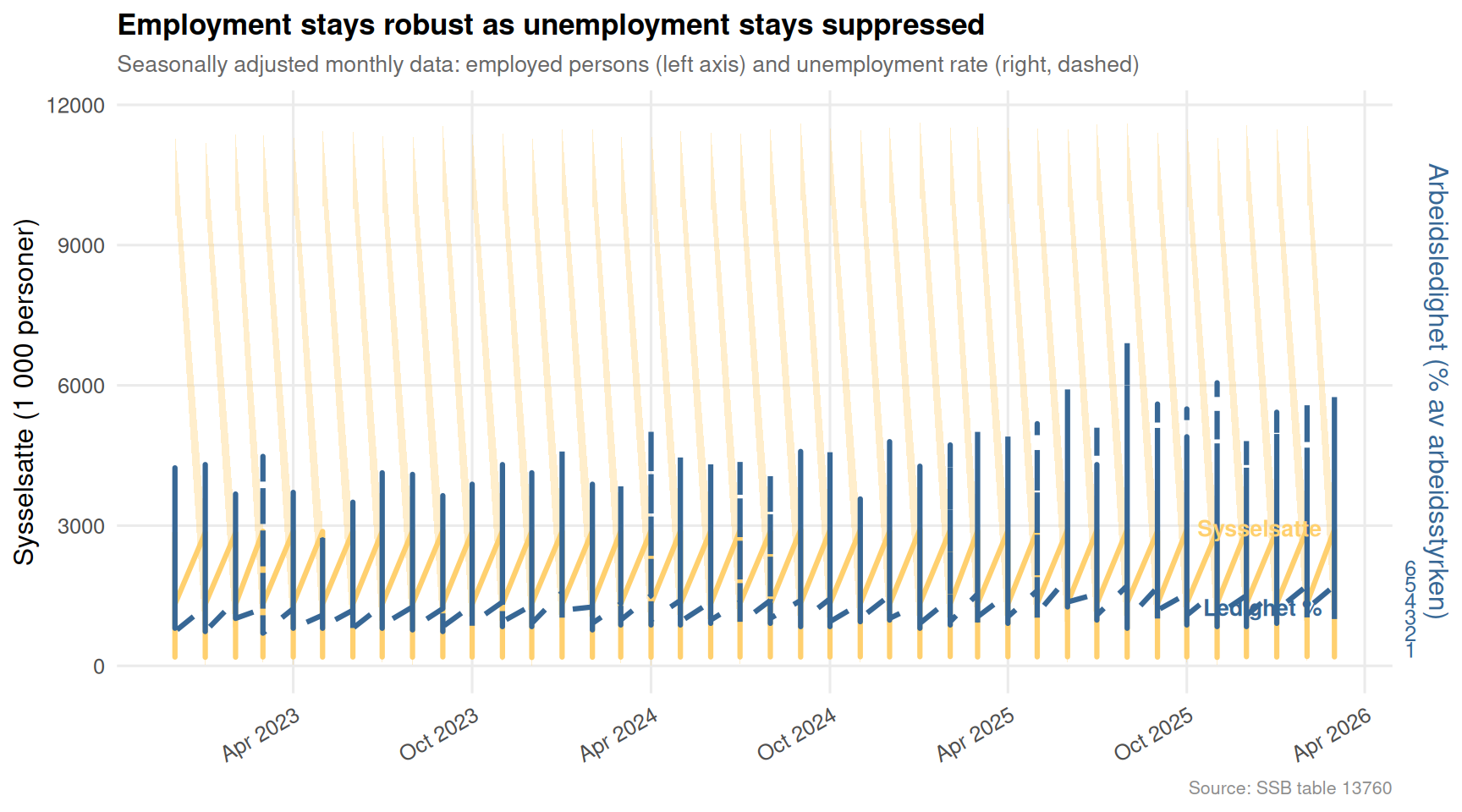
The area chart above tells the first part of the story. Seasonally adjusted employment has trended firmly upward over the past three years, while the unemployment rate has remained low and relatively stable. There is no sign of a labour market cracking under economic pressure — at least not yet.
if (!is.null(df2)) {

  series_col_df2  <- "vare- og tjenestegruppe"
  measure_col_df2 <- "statistikkvariabel"

  df2_12m <- df2 |>
    filter(.data[[measure_col_df2]] == "12-måneders endring (prosent)")

  if (nrow(df2_12m) == 0) {
    message("Filter empty. Values: ",
            paste(head(unique(df2[[measure_col_df2]]), 15), collapse = ", "))
    df2_12m <- NULL
  }

  if (!is.null(df2_12m)) {

    cats_to_show <- c(
      "I alt",
      "Matvarer og alkoholfrie drikkevarer",
      "Matvarer",
      "Brød og kornprodukter"
    )

    df2_ridge <- df2_12m |>
      filter(.data[[series_col_df2]] %in% cats_to_show) |>
      mutate(
        category = factor(.data[[series_col_df2]],
                          levels = rev(cats_to_show))
      )

    palette_ridge <- met.brewer("Hiroshige", n = 6)

    p2 <- ggplot(df2_ridge,
                 aes(x = value, y = category, fill = category)) +
      geom_density_ridges(
        alpha = 0.75, scale = 1.2,
        quantile_lines = TRUE, quantiles = 2,
        colour = "white", linewidth = 0.5
      ) +
      geom_vline(xintercept = 0, linetype = "dashed",
                 colour = "grey30", linewidth = 0.8) +
      scale_fill_manual(values = palette_ridge[c(1, 2, 4, 6)],
                        guide = "none") +
      scale_x_continuous(labels = function(x) paste0(x, "%"),
                         breaks = seq(-4, 14, 2)) +
      labs(
        title = "Food price inflation persistently above overall CPI",
        subtitle = "Distribution of monthly 12-month price changes across CPI categories (last 40 months)",
        x = "12-month change (%)",
        y = NULL,
        caption = "Source: SSB table 14700"
      ) +
      theme_minimal(base_size = 12) +
      theme(
        plot.title    = element_text(face = "bold", size = 13),
        plot.subtitle = element_text(size = 10, colour = "grey40"),
        plot.caption  = element_text(size = 8, colour = "grey55"),
        panel.grid.minor   = element_blank(),
        axis.text.y        = element_text(size = 10)
      )

    print(p2)
  }
}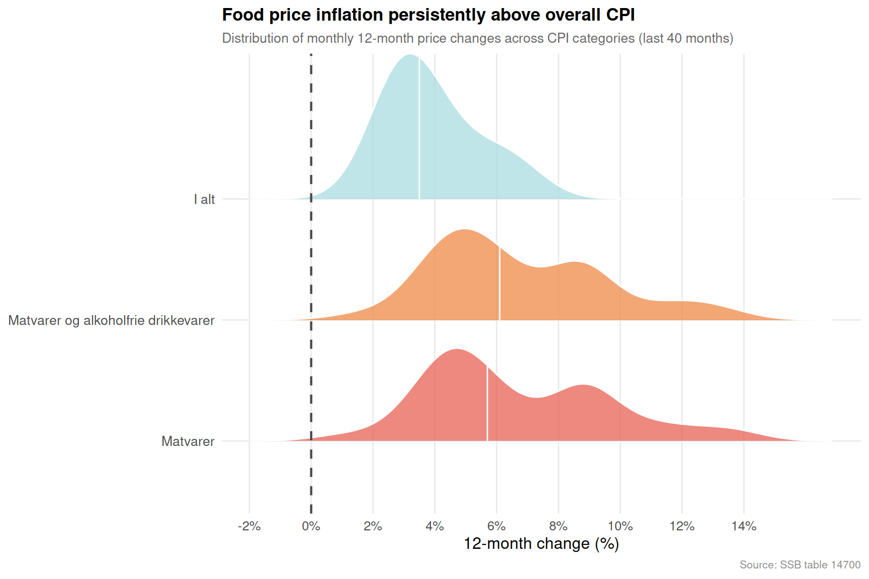
The ridgeline chart reveals where the inflation story becomes visceral. Food prices — and particularly bread and grain products — have shown a distribution of 12-month price changes skewed far to the right compared with the overall CPI. The median monthly reading for food items has been well above zero, with the mass of observations clustering between four and ten percent annual gains. For households that spend a disproportionate share of income on groceries, this is not an abstract statistic.
if (!is.null(df2)) {

  series_col_df2  <- "vare- og tjenestegruppe"
  measure_col_df2 <- "statistikkvariabel"

  df2_food_12m <- df2 |>
    filter(
      .data[[series_col_df2]]  == "Matvarer og alkoholfrie drikkevarer",
      .data[[measure_col_df2]] == "12-måneders endring (prosent)"
    )

  if (nrow(df2_food_12m) == 0) {
    message("Filter empty. Values: ",
            paste(head(unique(df2[[series_col_df2]]), 15), collapse = ", "))
    df2_food_12m <- NULL
  }

  df2_total_12m <- df2 |>
    filter(
      .data[[series_col_df2]]  == "I alt",
      .data[[measure_col_df2]] == "12-måneders endring (prosent)"
    )

  if (nrow(df2_total_12m) == 0) {
    message("Filter empty. Values: ",
            paste(head(unique(df2[[series_col_df2]]), 15), collapse = ", "))
    df2_total_12m <- NULL
  }

  if (!is.null(df2_food_12m) && !is.null(df2_total_12m)) {

    pal_lollipop <- met.brewer("Hiroshige", n = 7)

    df2_combined_lollipop <- bind_rows(
      df2_food_12m  |> mutate(series = "Matvarer og alkoholfrie drikkevarer"),
      df2_total_12m |> mutate(series = "KPI totalt (I alt)")
    ) |>
      arrange(date)

    # Take last 24 months for readability
    cutoff_date <- max(df2_combined_lollipop$date, na.rm = TRUE) %m-% months(23)
    df2_lollipop_sub <- df2_combined_lollipop |>
      filter(date >= cutoff_date)

    p3 <- ggplot(df2_lollipop_sub,
                 aes(x = date, y = value, colour = series)) +
      geom_segment(
        aes(xend = date, yend = 0),
        linewidth = 0.7, alpha = 0.6
      ) +
      geom_point(size = 2.8) +
      geom_hline(yintercept = 0, colour = "grey30", linewidth = 0.6) +
      geom_hline(yintercept = 2, colour = "grey60", linewidth = 0.5,
                 linetype = "dotted") +
      annotate("text", x = cutoff_date, y = 2.3,
               label = "2% target", size = 3, colour = "grey50",
               hjust = 0) +
      scale_colour_manual(
        values = c(
          "Matvarer og alkoholfrie drikkevarer" = pal_lollipop[5],
          "KPI totalt (I alt)"                  = pal_lollipop[2]
        ),
        name = NULL
      ) +
      scale_x_date(date_labels = "%b %Y", date_breaks = "3 months") +
      scale_y_continuous(labels = function(x) paste0(x, "%")) +
      facet_wrap(~ series, ncol = 1) +
      labs(
        title = "Food inflation repeatedly overshoots the headline CPI",
        subtitle = "12-month price change: food & non-alcoholic beverages vs. all-items CPI (last 24 months)",
        x = NULL,
        y = "12-month change (%)",
        caption = "Source: SSB table 14700. Dotted line = 2% reference."
      ) +
      theme_minimal(base_size = 12) +
      theme(
        plot.title    = element_text(face = "bold", size = 13),
        plot.subtitle = element_text(size = 10, colour = "grey40"),
        plot.caption  = element_text(size = 8, colour = "grey55"),
        legend.position  = "none",
        strip.text       = element_text(face = "bold", size = 10),
        axis.text.x      = element_text(angle = 30, hjust = 1),
        panel.grid.minor = element_blank()
      )

    print(p3)
  }
}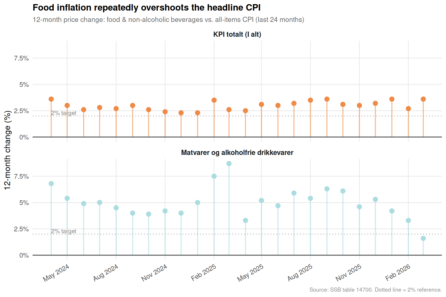
When broken out month by month, the contrast is stark. Food price inflation has rarely dipped near the two percent target that most central banks treat as an anchor for expectations. The all-items headline has been volatile but has trended lower; food has been stickier. This divergence matters because low-income households allocate a much larger share of their budgets to groceries than high-income ones, meaning the pain is unevenly distributed across the income scale.
if (!is.null(df3)) {

  series_col_df3  <- "makrostørrelse"
  measure_col_df3 <- "statistikkvariabel"

  # Volume change for household consumption and public consumption
  df3_vol <- df3 |>
    filter(
      .data[[series_col_df3]] %in% c(
        "Konsum i husholdninger og ideelle organisasjoner",
        "Konsum i offentlig forvaltning"
      ),
      .data[[measure_col_df3]] == "Volumendring, årlig (prosent)"
    )

  if (nrow(df3_vol) == 0) {
    message("Filter empty. Values: ",
            paste(head(unique(df3[[series_col_df3]]), 15), collapse = ", "))
    df3_vol <- NULL
  }

  if (!is.null(df3_vol)) {

    pal_slope <- met.brewer("Hiroshige", n = 7)

    df3_vol <- df3_vol |>
      mutate(
        year = lubridate::year(date),
        label_series = case_when(
          .data[[series_col_df3]] == "Konsum i husholdninger og ideelle organisasjoner" ~ "Husholdninger",
          .data[[series_col_df3]] == "Konsum i offentlig forvaltning"                   ~ "Offentlig forvaltning",
          TRUE ~ .data[[series_col_df3]]
        )
      )

    recent_years <- df3_vol |>
      filter(year >= max(year, na.rm = TRUE) - 9)

    p4 <- ggplot(recent_years,
                 aes(x = year, y = value,
                     colour = label_series,
                     group  = label_series)) +
      geom_hline(yintercept = 0, colour = "grey40",
                 linewidth = 0.7, linetype = "dashed") +
      geom_line(linewidth = 1.3) +
      geom_point(size = 3) +
      geom_text(
        data = recent_years |> filter(year == max(year)),
        aes(label = paste0(label_series, "\n", round(value, 1), "%")),
        hjust = -0.08, size = 3.2, fontface = "bold"
      ) +
      scale_colour_manual(
        values = c(
          "Husholdninger"         = pal_slope[2],
          "Offentlig forvaltning" = pal_slope[5]
        ),
        guide = "none"
      ) +
      scale_x_continuous(
        breaks = seq(min(recent_years$year), max(recent_years$year), 1),
        expand = expansion(mult = c(0.02, 0.25))
      ) +
      scale_y_continuous(labels = function(x) paste0(x, "%")) +
      labs(
        title = "Household consumption volumes squeezed — public spending diverges",
        subtitle = "Annual volume change (%) in household vs. government consumption; national accounts, fixed 2023 prices",
        x = NULL,
        y = "Volume change, annual (%)",
        caption = "Source: SSB table 09189"
      ) +
      theme_minimal(base_size = 12) +
      theme(
        plot.title    = element_text(face = "bold", size = 13),
        plot.subtitle = element_text(size = 10, colour = "grey40"),
        plot.caption  = element_text(size = 8, colour = "grey55"),
        panel.grid.minor  = element_blank(),
        axis.text.x       = element_text(angle = 30, hjust = 1)
      )

    print(p4)
  }
}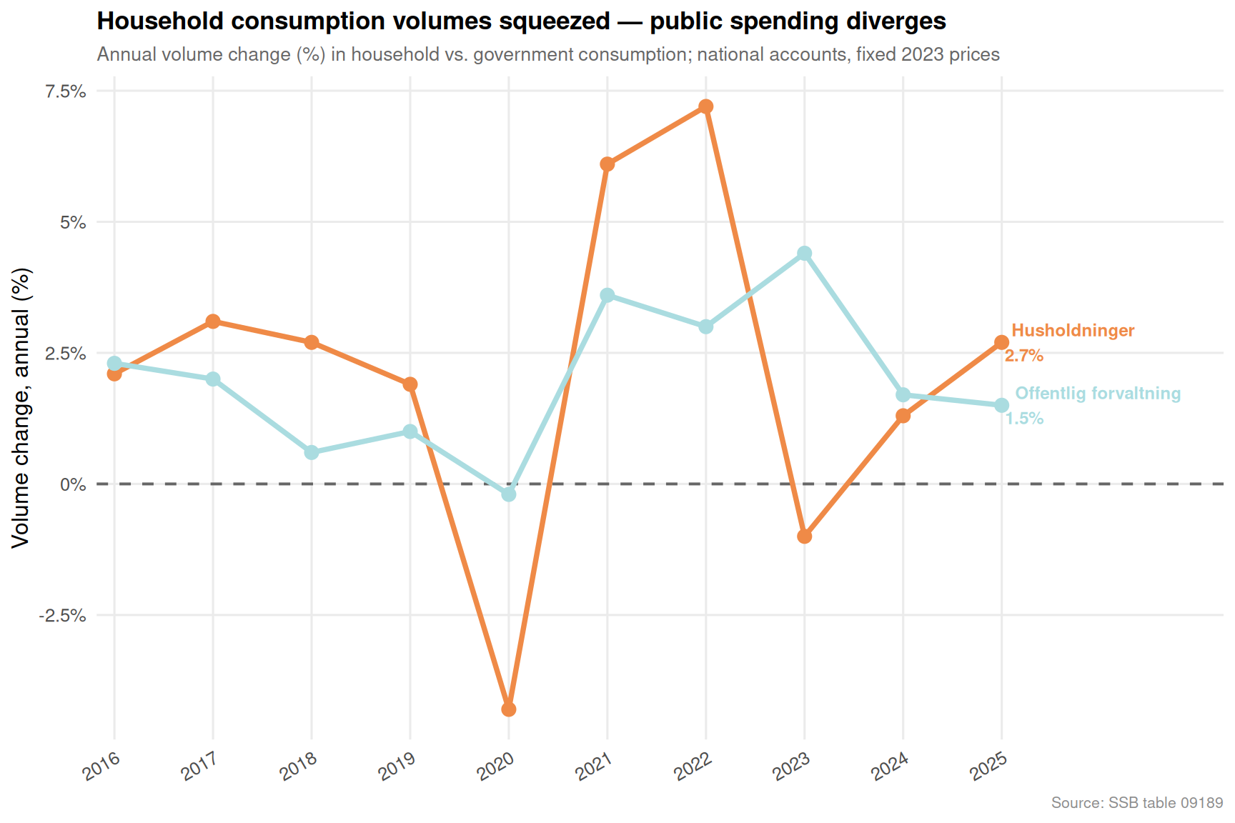
The slope chart delivers the national accounts verdict. Household consumption in real volume terms has decelerated sharply and in recent years has barely registered positive growth. Government consumption, by contrast, has been considerably more resilient — a reflection of Norway’s continued fiscal capacity thanks to petroleum revenues. This divergence encapsulates the paradox: the public sector keeps hiring and spending, employment holds up, but private households are running on empty.
if (!is.null(df3)) {

  series_col_df3  <- "makrostørrelse"
  measure_col_df3 <- "statistikkvariabel"

  df3_price_vol <- df3 |>
    filter(
      .data[[series_col_df3]] %in% c(
        "Varekonsum",
        "Tjenestekonsum"
      ),
      .data[[measure_col_df3]] %in% c(
        "Volumendring, årlig (prosent)",
        "Prisendring, årlig (prosent)"
      )
    ) |>
    mutate(
      year = lubridate::year(date),
      category = case_when(
        .data[[series_col_df3]] == "Varekonsum"     ~ "Goods consumption",
        .data[[series_col_df3]] == "Tjenestekonsum" ~ "Services consumption",
        TRUE ~ .data[[series_col_df3]]
      ),
      change_type = case_when(
        .data[[measure_col_df3]] == "Volumendring, årlig (prosent)" ~ "Volume change",
        .data[[measure_col_df3]] == "Prisendring, årlig (prosent)"  ~ "Price change",
        TRUE ~ .data[[measure_col_df3]]
      )
    )

  if (nrow(df3_price_vol) == 0) {
    message("Filter empty. Values: ",
            paste(head(unique(df3[[series_col_df3]]), 15), collapse = ", "))
    df3_price_vol <- NULL
  }

  if (!is.null(df3_price_vol)) {

    # Last 5 years for dumbbell
    df3_db <- df3_price_vol |>
      filter(year >= max(year, na.rm = TRUE) - 4) |>
      select(year, category, change_type, value) |>
      pivot_wider(names_from = change_type, values_from = value) |>
      filter(!is.na(`Volume change`), !is.na(`Price change`))

    pal_db <- met.brewer("Hiroshige", n = 7)

    p5 <- ggplot(df3_db, aes(y = factor(year))) +
      geom_segment(
        aes(x = `Volume change`, xend = `Price change`,
            y = factor(year), yend = factor(year)),
        colour = "grey70", linewidth = 1.5
      ) +
      geom_point(aes(x = `Volume change`, colour = "Volume change"),
                 size = 4) +
      geom_point(aes(x = `Price change`, colour = "Price change"),
                 size = 4) +
      geom_vline(xintercept = 0, colour = "grey30",
                 linewidth = 0.7, linetype = "dashed") +
      scale_colour_manual(
        values = c(
          "Volume change" = pal_db[2],
          "Price change"  = pal_db[5]
        ),
        name = NULL
      ) +
      scale_x_continuous(labels = function(x) paste0(x, "%")) +
      facet_wrap(~ category, ncol = 2) +
      labs(
        title = "Prices soar; volumes stagnate — the household squeeze in numbers",
        subtitle = "Annual price change vs. volume change for goods and services consumption (dumbbell: price = orange, volume = blue)",
        x = "Annual change (%)",
        y = NULL,
        caption = "Source: SSB table 09189"
      ) +
      theme_minimal(base_size = 12) +
      theme(
        plot.title    = element_text(face = "bold", size = 13),
        plot.subtitle = element_text(size = 10, colour = "grey40"),
        plot.caption  = element_text(size = 8, colour = "grey55"),
        legend.position  = "bottom",
        strip.text       = element_text(face = "bold", size = 10),
        panel.grid.minor = element_blank()
      )

    print(p5)
  }
}
The dumbbell chart closes the analytical loop. For both goods and services consumption, price increases (orange dots) have consistently outpaced volume changes (blue dots) in recent years. The gap is the real wage squeeze made visible: households are paying more but getting less in physical terms. Goods consumption — more exposed to global commodity prices and import costs — shows the widest dumbbell spans.
Employment held firm. Seasonally adjusted employment has grown steadily over the observation window, and the unemployment rate remained suppressed well below levels seen in most comparable European economies.
Food inflation was persistent and above headline. The 12-month price change for food and non-alcoholic beverages consistently exceeded the all-items CPI across the distribution of monthly readings, with the bulk of observations clustering between four and ten percent annual gains.
Household consumption volumes stagnated. Real volume growth in household consumption — measured at fixed 2023 prices — decelerated sharply and hovered near zero in the most recent years, even as current-price figures appeared more buoyant.
Public sector consumption diverged. Government consumption volumes held up considerably better than private household spending, reflecting Norway’s unique fiscal position but also raising questions about whether public sector activity is masking underlying private sector weakness.
The price-volume gap widened most for goods. In both goods and services categories, price changes outstripped volume changes, but the divergence was most extreme for goods — the category most exposed to international commodity and energy price cycles.
Norway’s economic paradox in 2026 is not a contradiction so much as a two-speed economy. The public sector and energy-adjacent industries sustain employment, wages, and even GDP aggregates. But behind those headline numbers, private households are facing a cost squeeze that has few recent precedents. When food prices rise faster than wages and real consumption volumes stagnate, the human experience of the economy diverges sharply from what aggregate employment figures suggest.
The deeper question is whether this can persist. Historically, labour markets eventually respond to prolonged consumption weakness — through reduced hours, hiring freezes, or outright job losses in consumer-facing industries. Norway’s petroleum buffer has bought time, but it cannot indefinitely insulate households from the arithmetic of inflation exceeding real income growth. The data assembled here suggest that the reckoning, while delayed, has been quietly underway for some time.