Code
library(tidyverse)
library(lubridate)
library(PxWebApiData)
library(scales)
library(MetBrewer)
library(ggridges)library(tidyverse)
library(lubridate)
library(PxWebApiData)
library(scales)
library(MetBrewer)
library(ggridges)df1 <- NULL
tryCatch({
raw <- ApiData(
"https://data.ssb.no/api/v0/no/table/09429",
Region = TRUE,
Nivaa = TRUE,
Kjonn = TRUE,
ContentsCode = TRUE,
Tid = list(filter = "top", values = 40)
)
tmp <- raw[[1]]
time_col <- "år"
value_col <- "value"
series_col <- "nivå"
measure_col <- "statistikkvariabel"
df1 <- tmp |>
mutate(
value = as.numeric(.data[[value_col]]),
time_str = .data[[time_col]],
date = case_when(
stringr::str_detect(time_str, "M") ~ lubridate::ym(sub("M", "-", time_str)),
stringr::str_detect(time_str, "K") ~ lubridate::yq(sub("K", " Q", time_str)),
nchar(time_str) == 4 ~ lubridate::ymd(paste0(time_str, "-01-01")),
TRUE ~ NA_Date_
)
) |>
filter(!is.na(value), !is.na(date))
}, error = function(e) message("Fetch failed: ", e$message))df2 <- NULL
tryCatch({
raw <- ApiData(
"https://data.ssb.no/api/v0/no/table/05110",
ArbStyrkStatus = TRUE,
Kjonn = TRUE,
Alder = TRUE,
ContentsCode = TRUE,
Tid = list(filter = "top", values = 40)
)
tmp <- raw[[1]]
time_col <- "kvartal"
value_col <- "value"
series_col <- "arbeidsstyrkestatus"
measure_col <- "statistikkvariabel"
df2 <- tmp |>
mutate(
value = as.numeric(.data[[value_col]]),
time_str = .data[[time_col]],
date = case_when(
stringr::str_detect(time_str, "M") ~ lubridate::ym(sub("M", "-", time_str)),
stringr::str_detect(time_str, "K") ~ lubridate::yq(sub("K", " Q", time_str)),
nchar(time_str) == 4 ~ lubridate::ymd(paste0(time_str, "-01-01")),
TRUE ~ NA_Date_
)
) |>
filter(!is.na(value), !is.na(date))
}, error = function(e) message("Fetch failed: ", e$message))df3 <- NULL
tryCatch({
raw <- ApiData(
"https://data.ssb.no/api/v0/no/table/10634",
Region = TRUE,
HovedlovbruddKrim = TRUE,
Alder = TRUE,
ContentsCode = TRUE,
Tid = list(filter = "top", values = 40)
)
tmp <- raw[[1]]
time_col <- "år"
value_col <- "value"
series_col <- "hovedlovbruddstype"
measure_col <- "statistikkvariabel"
df3 <- tmp |>
mutate(
value = as.numeric(.data[[value_col]]),
time_str = .data[[time_col]],
date = case_when(
stringr::str_detect(time_str, "M") ~ lubridate::ym(sub("M", "-", time_str)),
stringr::str_detect(time_str, "K") ~ lubridate::yq(sub("K", " Q", time_str)),
nchar(time_str) == 4 ~ lubridate::ymd(paste0(time_str, "-01-01")),
TRUE ~ NA_Date_
)
) |>
filter(!is.na(value), !is.na(date))
}, error = function(e) message("Fetch failed: ", e$message))Norway has spent the past decade pushing more of its population into higher education. Between 2017 and 2024, university and college enrolment climbed year after year, driven by government ambition, a knowledge-economy narrative, and the simple logic that qualifications protect against unemployment. Yet over the same period, the labour force participation rate barely budged, the number of people outside the workforce remained stubbornly large, and the total employed population grew only modestly. Something does not add up. If degrees are the answer, what is the question? This post puts three SSB datasets in conversation to probe what Norway’s education expansion has actually delivered — and what it may have obscured.
Norway’s enrolment surge was not evenly spread across qualification levels. Short university and college programmes absorbed the bulk of growth, but the longer academic degrees also expanded significantly. Looking at the national totals by level — and disaggregating by gender — reveals a structural shift in who Norwegian society is now educating.
if (!is.null(df1)) {
  # Filter for national totals (all regions), persons 16+, and the main education levels
  series_col_df1 <- "nivå"
  measure_col_df1 <- "statistikkvariabel"

  levels_interest <- c(
    "Universitets- og høgskolenivå, kort",
    "Universitets- og høgskolenivå, lang",
    "Fagskolenivå"
  )

  df1_area <- df1 |>
    filter(
      .data[[measure_col_df1]] == "Personer 16 år og over",
      .data[[series_col_df1]] %in% levels_interest
    )

  if (nrow(df1_area) == 0) {
    message("Filter empty. Values: ", paste(head(unique(df1[[series_col_df1]]), 15), collapse = ", "))
    df1_area <- NULL
  }

  if (!is.null(df1_area)) {
    # Aggregate across all regions and genders to get national totals
    df1_agg <- df1_area |>
      group_by(date, .data[[series_col_df1]]) |>
      summarise(total = sum(value, na.rm = TRUE), .groups = "drop") |>
      rename(level = 2)

    # Shorten labels
    df1_agg <- df1_agg |>
      mutate(level_short = case_when(
        level == "Universitets- og høgskolenivå, kort" ~ "University/college, short",
        level == "Universitets- og høgskolenivå, lang" ~ "University/college, long",
        level == "Fagskolenivå"                        ~ "Vocational college",
        TRUE ~ level
      ))

    pal <- MetBrewer::met.brewer("Hiroshige", n = 3)

    p1 <- ggplot(df1_agg, aes(x = date, y = total / 1000, fill = level_short)) +
      geom_area(alpha = 0.85, colour = "white", linewidth = 0.3) +
      scale_fill_manual(values = pal, name = NULL) +
      scale_x_date(date_breaks = "1 year", date_labels = "%Y") +
      scale_y_continuous(labels = label_comma(suffix = "k")) +
      labs(
        title = "Norway's higher education expansion, 2017-2024",
        subtitle = "Short university programmes dominate enrolment growth; vocational colleges remain marginal",
        x = NULL,
        y = "Students (thousands)",
        caption = "Source: SSB table 09429"
      ) +
      theme_minimal(base_size = 12) +
      theme(
        legend.position = "bottom",
        panel.grid.minor = element_blank(),
        plot.title = element_text(face = "bold"),
        plot.subtitle = element_text(colour = "grey40"),
        axis.text.x = element_text(angle = 30, hjust = 1)
      )

    print(p1)
  }
}
The stacked area chart makes the hierarchy plain: short-cycle university and college programmes account for the overwhelming majority of enrolment, and it is here that growth has been concentrated. Vocational college (fagskolenivå) enrolment is comparatively tiny, which is a recurring political headache — Norway has long struggled to persuade school-leavers that skilled trades offer a credible career path.
One of the most striking features of Norwegian higher education is the widening gap between male and female enrolment. Women now outnumber men at university by a substantial margin — a reversal of historical norms that has prompted concern about what is happening to young men in the Norwegian labour market.
if (!is.null(df1)) {
  series_col_df1  <- "nivå"
  measure_col_df1 <- "statistikkvariabel"

  df1_gender <- df1 |>
    filter(
      .data[[measure_col_df1]] == "Personer 16 år og over",
      .data[[series_col_df1]] == "Universitets- og høgskolenivå, kort"
    )

  if (nrow(df1_gender) == 0) {
    message("Filter empty. Values: ", paste(head(unique(df1[[series_col_df1]]), 15), collapse = ", "))
    df1_gender <- NULL
  }

  if (!is.null(df1_gender)) {
    # Focus on national level, split by gender
    # Check what the gender column is called
    gender_col <- names(df1_gender)[grepl("kj.nn|gender", names(df1_gender), ignore.case = TRUE)][1]

    if (is.na(gender_col)) stop("Cannot detect column: ", paste(names(df1_gender), collapse = ", "))

    # Summarise nationally by year and gender
    df1_gend_nat <- df1_gender |>
      group_by(year = lubridate::year(date), gender = .data[[gender_col]]) |>
      summarise(total = sum(value, na.rm = TRUE), .groups = "drop") |>
      filter(gender %in% c("Menn", "Kvinner"))

    if (nrow(df1_gend_nat) > 0) {
      df1_gend_wide <- df1_gend_nat |>
        pivot_wider(names_from = gender, values_from = total) |>
        filter(!is.na(Menn), !is.na(Kvinner)) |>
        mutate(gap = Kvinner - Menn)

      pal2 <- MetBrewer::met.brewer("Hiroshige", n = 5)
      col_women <- pal2[1]
      col_men   <- pal2[5]

      p2 <- ggplot(df1_gend_wide, aes(y = factor(year))) +
        geom_segment(aes(x = Menn / 1000, xend = Kvinner / 1000,
                         yend = factor(year)),
                     colour = "grey70", linewidth = 1.2) +
        geom_point(aes(x = Menn / 1000), colour = col_men, size = 4) +
        geom_point(aes(x = Kvinner / 1000), colour = col_women, size = 4) +
        geom_text(aes(x = (Menn + Kvinner) / 2 / 1000,
                      label = paste0("+", round(gap / 1000, 0), "k women")),
                  vjust = -0.8, size = 3, colour = "grey30") +
        annotate("text", x = Inf, y = 1,
                 label = paste0("Men"),
                 hjust = 1.2, colour = col_men, fontface = "bold", size = 3.5) +
        scale_x_continuous(labels = label_comma(suffix = "k")) +
        labs(
          title = "Women outnumber men in short university programmes",
          subtitle = "The gender gap in short-cycle higher education has widened every year since 2017",
          x = "Students (thousands)",
          y = NULL,
          caption = "Source: SSB table 09429"
        ) +
        theme_minimal(base_size = 12) +
        theme(
          panel.grid.minor = element_blank(),
          panel.grid.major.y = element_blank(),
          plot.title = element_text(face = "bold"),
          plot.subtitle = element_text(colour = "grey40")
        )

      print(p2)
    }
  }
}
The dumbbell chart exposes a steady drift: each year the gap between the left dot (men) and right dot (women) widens. By 2024, Norwegian women enrolled in short university programmes outnumber men by tens of thousands. This matters for the labour market story because male school-leavers who do not enter higher education are disproportionately the ones who end up outside the workforce entirely.
If education were smoothly translating into employment, we would expect to see the workforce participation rate rising in tandem with enrolment. The quarterly labour force survey data allows us to track the employed, unemployed, and those entirely outside the labour market over recent years.
if (!is.null(df2)) {
  series_col_df2  <- "arbeidsstyrkestatus"
  measure_col_df2 <- "statistikkvariabel"

  # Pull employed and outside-labour-force counts, all ages and genders combined
  statuses <- c("Sysselsatte", "Personer utenfor arbeidsstyrken", "Arbeidsledige")

  df2_sub <- df2 |>
    filter(
      .data[[measure_col_df2]] == "Personer (1 000 personer)",
      .data[[series_col_df2]] %in% statuses
    )

  if (nrow(df2_sub) == 0) {
    message("Filter empty. Values: ", paste(head(unique(df2[[series_col_df2]]), 15), collapse = ", "))
    df2_sub <- NULL
  }

  if (!is.null(df2_sub)) {
    # Aggregate across gender and age to get total national figures per quarter
    df2_agg <- df2_sub |>
      group_by(date, status = .data[[series_col_df2]]) |>
      summarise(total = sum(value, na.rm = TRUE), .groups = "drop")

    # Shorten status labels
    df2_agg <- df2_agg |>
      mutate(status_short = case_when(
        status == "Sysselsatte"                     ~ "Employed",
        status == "Personer utenfor arbeidsstyrken" ~ "Outside labour force",
        status == "Arbeidsledige"                   ~ "Unemployed",
        TRUE ~ status
      ))

    # Keep only last 10 years
    df2_recent <- df2_agg |>
      filter(date >= as.Date("2015-01-01"))

    pal3 <- MetBrewer::met.brewer("Hiroshige", n = 3)

    p3 <- ggplot(df2_recent, aes(x = date, y = total, colour = status_short)) +
      geom_line(linewidth = 1.1) +
      geom_point(data = df2_recent |> filter(date == max(date)),
                 size = 3) +
      ggrepel::geom_text_repel(
        data = df2_recent |> filter(date == max(date)),
        aes(label = paste0(status_short, "\n", round(total, 0), "k")),
        size = 3, nudge_x = 60, direction = "y", segment.colour = "grey70"
      ) +
      scale_colour_manual(values = pal3, guide = "none") +
      scale_x_date(date_breaks = "1 year", date_labels = "%Y") +
      scale_y_continuous(labels = label_comma(suffix = "k")) +
      labs(
        title = "Employment and inactivity in Norway, 2015-2025",
        subtitle = "Employed numbers grew modestly; the pool outside the labour force remains persistently large",
        x = NULL,
        y = "Persons (thousands)",
        caption = "Source: SSB table 05110"
      ) +
      theme_minimal(base_size = 12) +
      theme(
        panel.grid.minor = element_blank(),
        plot.title = element_text(face = "bold"),
        plot.subtitle = element_text(colour = "grey40"),
        axis.text.x = element_text(angle = 30, hjust = 1)
      )

    print(p3)
  }
}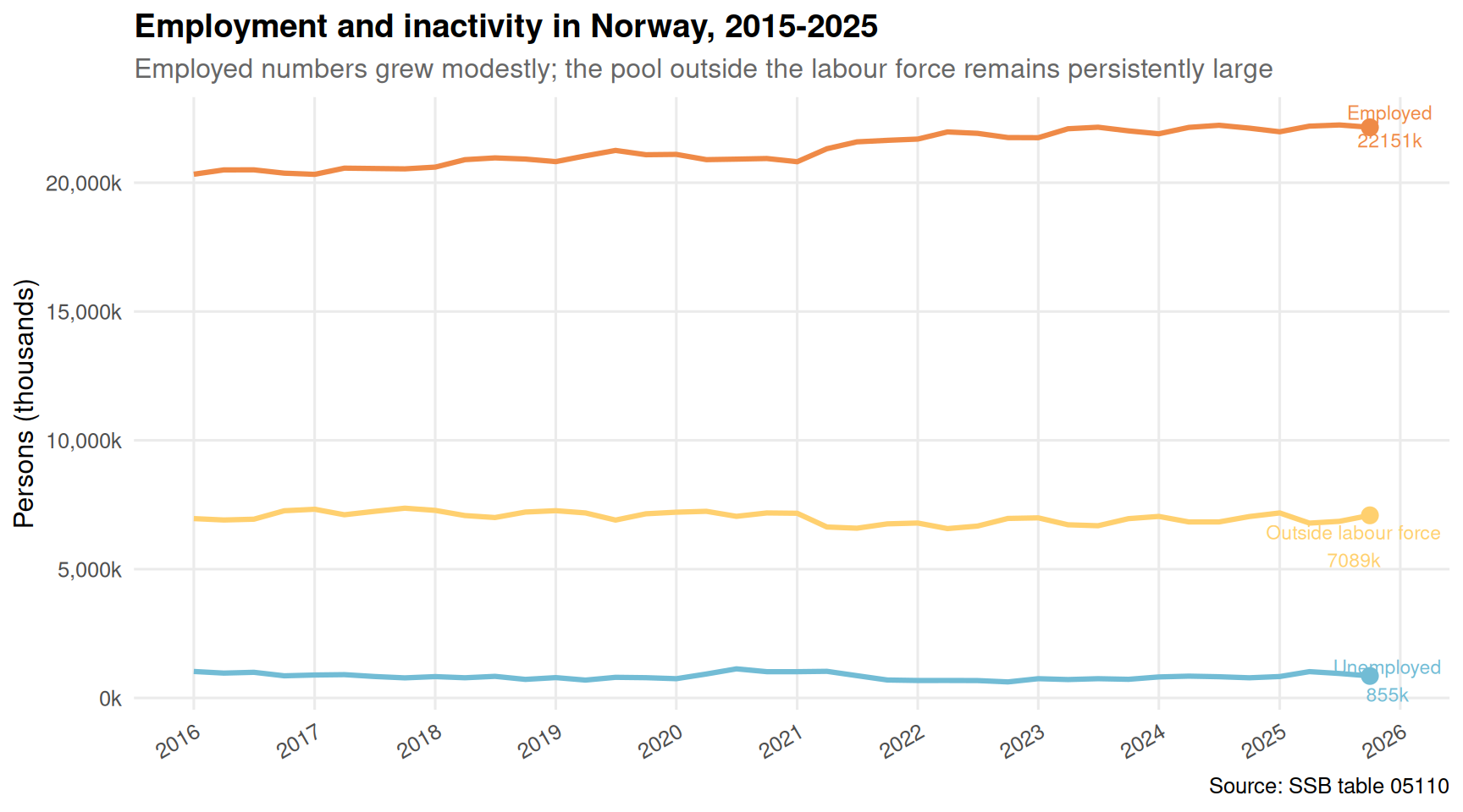
The line chart tells a sobering story. Employment did rise after the pandemic shock, but the group outside the labour force entirely — neither employed nor actively seeking work — has remained enormous and barely compressed. This is the reservoir of people that education policy implicitly targets, yet the numbers suggest the pipeline from classroom to workplace is far from seamless.
A society that expands education while failing to absorb graduates into productive work creates friction. One downstream signal is the criminal justice system. The SSB’s sentencing data captures which age groups and crime types are generating the most sentences — and whether the picture has changed as education enrolment has risen.
if (!is.null(df3)) {
  series_col_df3  <- "hovedlovbruddstype"
  measure_col_df3 <- "statistikkvariabel"

  df3_sub <- df3 |>
    filter(
      .data[[measure_col_df3]] == "Straffede personer per 1000 innbyggere",
      .data[[series_col_df3]] == "Alle lovbruddsgrupper (ekskl. Trafikkovertredelse)"
    )

  if (nrow(df3_sub) == 0) {
    message("Filter empty. Values: ", paste(head(unique(df3[[series_col_df3]]), 15), collapse = ", "))
    df3_sub <- NULL
  }

  if (!is.null(df3_sub)) {
    # Look at age-group breakdown; find the age column
    age_col <- names(df3_sub)[grepl("alder|age", names(df3_sub), ignore.case = TRUE)][1]

    if (is.na(age_col)) stop("Cannot detect column: ", paste(names(df3_sub), collapse = ", "))

    df3_heat <- df3_sub |>
      group_by(year = lubridate::year(date), age = .data[[age_col]]) |>
      summarise(rate = mean(value, na.rm = TRUE), .groups = "drop") |>
      filter(!is.na(rate), rate > 0)

    # Remove catch-all age groups for clarity
    df3_heat <- df3_heat |>
      filter(!age %in% c("Alle aldre", "15 år og over"))

    if (nrow(df3_heat) > 0) {
      pal4 <- MetBrewer::met.brewer("Hiroshige", type = "continuous")

      p4 <- ggplot(df3_heat, aes(x = factor(year), y = age, fill = rate)) +
        geom_tile(colour = "white", linewidth = 0.4) +
        geom_text(aes(label = round(rate, 1)), size = 2.8, colour = "white") +
        scale_fill_gradientn(
          colours = MetBrewer::met.brewer("Hiroshige", n = 9, type = "continuous"),
          name = "Sentenced\nper 1,000"
        ) +
        labs(
          title = "Sentencing rates by age group, 2013-2020",
          subtitle = "Young men in their 20s carry the highest sentencing burden — the same cohort least likely to complete higher education",
          x = NULL,
          y = "Age group",
          caption = "Source: SSB table 10634 (excl. traffic offences)"
        ) +
        theme_minimal(base_size = 11) +
        theme(
          panel.grid = element_blank(),
          plot.title = element_text(face = "bold"),
          plot.subtitle = element_text(colour = "grey40"),
          axis.text.y = element_text(size = 9)
        )

      print(p4)
    }
  }
}
The heatmap reveals a persistent concentration of sentencing among young adults in their early twenties — precisely the cohort that is most likely to be male, and least likely to have entered higher education. The rate per 1,000 inhabitants in this age band dwarfs every other group. While Norway’s overall crime trajectory is downward (well-documented in other analyses), the age structure of sentencing has remained stubbornly stable, suggesting that the young men left behind by the education expansion are not quietly disappearing into productive work.
To complete the picture, it is worth quantifying not just the absolute size of each education level but its percentage growth since 2017. Which programmes actually expanded, and by how much?
if (!is.null(df1)) {
  series_col_df1  <- "nivå"
  measure_col_df1 <- "statistikkvariabel"

  df1_growth <- df1 |>
    filter(
      .data[[measure_col_df1]] == "Personer 16 år og over"
    )

  if (nrow(df1_growth) == 0) {
    message("Filter empty. Values: ", paste(head(unique(df1[[measure_col_df1]]), 15), collapse = ", "))
    df1_growth <- NULL
  }

  if (!is.null(df1_growth)) {
    # National aggregate by level and year
    df1_g2 <- df1_growth |>
      group_by(year = lubridate::year(date), level = .data[[series_col_df1]]) |>
      summarise(total = sum(value, na.rm = TRUE), .groups = "drop")

    # Keep only meaningful education levels (exclude catch-all)
    df1_g2 <- df1_g2 |>
      filter(!level %in% c("Utdanningsniv. i alt", "Grunnskoleniv.",
                            "Videregj.ende skoleniv."))

    # Compute growth from earliest to latest year
    df1_endpoints <- df1_g2 |>
      group_by(level) |>
      filter(year == min(year) | year == max(year)) |>
      arrange(level, year) |>
      summarise(
        start_year = first(year),
        end_year   = last(year),
        start_val  = first(total),
        end_val    = last(total),
        pct_change = (last(total) - first(total)) / first(total) * 100,
        .groups = "drop"
      ) |>
      filter(start_val > 0)

    # Shorten labels
    df1_endpoints <- df1_endpoints |>
      mutate(level_short = case_when(
        level == "Universitets- og høgskolenivå, kort" ~ "University/college,\nshort cycle",
        level == "Universitets- og høgskolenivå, lang" ~ "University/college,\nlong cycle",
        level == "Fagskolenivå"                        ~ "Vocational\ncollege",
        TRUE ~ level
      )) |>
      arrange(pct_change)

    pal5 <- MetBrewer::met.brewer("Hiroshige", n = nrow(df1_endpoints))

    p5 <- ggplot(df1_endpoints,
                 aes(x = pct_change, y = reorder(level_short, pct_change))) +
      geom_segment(aes(x = 0, xend = pct_change,
                       yend = reorder(level_short, pct_change)),
                   colour = "grey70", linewidth = 1) +
      geom_point(aes(colour = level_short), size = 5) +
      geom_text(aes(label = paste0("+", round(pct_change, 1), "%")),
                hjust = -0.3, size = 3.5, colour = "grey20") +
      scale_colour_manual(values = pal5, guide = "none") +
      scale_x_continuous(
        labels = label_percent(scale = 1),
        expand = expansion(mult = c(0, 0.25))
      ) +
      geom_vline(xintercept = 0, colour = "grey40", linetype = "dashed") +
      labs(
        title = paste0("Enrolment growth by education level, ",
                       min(df1_endpoints$start_year), "-",
                       max(df1_endpoints$end_year)),
        subtitle = "Vocational college and long-cycle university programmes grew fastest in relative terms",
        x = "Percentage change in enrolment",
        y = NULL,
        caption = "Source: SSB table 09429"
      ) +
      theme_minimal(base_size = 12) +
      theme(
        panel.grid.minor = element_blank(),
        panel.grid.major.y = element_blank(),
        plot.title = element_text(face = "bold"),
        plot.subtitle = element_text(colour = "grey40")
      )

    print(p5)
  }
}
The lollipop chart adds nuance to the expansion narrative. In relative percentage terms, long-cycle university programmes and vocational colleges may have grown from smaller bases, even if short-cycle programmes dominate in absolute numbers. The divergence between relative and absolute growth rates is itself a policy story: policymakers who celebrate percentage increases in vocational enrolment can simultaneously watch the absolute vocational total remain a rounding error next to the university mass.
Enrolment in short-cycle university and college programmes in Norway has grown every year from 2017 to 2024, making it the dominant form of post-secondary education by a wide margin over vocational college pathways.
Women outnumber men in short-cycle higher education by a gap that has widened annually, reaching tens of thousands of students — a structural gender asymmetry with profound implications for which workers enter which sectors.
The pool of working-age people outside the Norwegian labour force entirely remains very large and has not materially compressed despite rising education levels and a post-pandemic employment recovery, suggesting that more degrees have not automatically converted the inactive into the active.
Young adults in their early to mid-twenties carry the highest sentencing rate per 1,000 inhabitants — a cohort that overlaps with those least likely to have completed higher education, pointing to an unresolved connection between educational exclusion and justice-system contact.
In relative growth terms, long-cycle academic programmes expanded from their smaller base at a pace that deserves attention: Norway is quietly producing more PhDs and master’s graduates even as the broad economy’s capacity to absorb them remains uncertain.
Norway’s education-employment paradox is not unique, but the Norwegian version has a particular sharpness. A country with a sovereign wealth fund larger than any other on the planet, and a welfare state designed to catch those who fall, should in theory be well-placed to translate mass education into mass productivity. That it has not done so cleanly suggests the bottleneck is not financial. It may be structural: an economy whose most productive sector — petroleum — employs relatively few people and whose public sector has finite absorption capacity, leaving a large and growing population of educated young workers competing for a constrained set of knowledge-economy jobs. The students keep enrolling. The question of what they do after graduating deserves far more attention than the enrolment statistics alone can provide.