Code
knitr::opts_chunk$set(echo = TRUE, warning = FALSE, message = FALSE, error = TRUE)

library(tidyverse)
library(PxWebApiData)
library(lubridate)
library(scales)
library(MetBrewer)
library(ggridges)

pal <- met.brewer("Hokusai1", 7)Norway’s welfare state runs on tax revenue, but the composition of who pays what has shifted dramatically over the past two decades. Using fresh SSB data on general government revenue and expenditure, we can see which sectors of the economy have become the fiscal backbone—and which have faded as contributors.
knitr::opts_chunk$set(echo = TRUE, warning = FALSE, message = FALSE, error = TRUE)
library(tidyverse)
library(PxWebApiData)
library(lubridate)
library(scales)
library(MetBrewer)
library(ggridges)
pal <- met.brewer("Hokusai1", 7)We’ll fetch annual general government revenue data (table 10948) across different economic sectors. The data shows how much each sector—from households to financial corporations to non-financial enterprises—contributes to public coffers through various revenue streams.
df <- NULL

tryCatch({
  raw <- ApiData(
    "https://data.ssb.no/api/v0/no/table/10948",
    Eiersektor = TRUE,
    ContentsCode = TRUE,
    Tid = list(filter = "top", values = 40)
  )
  tmp <- raw[[1]]
  message("Columns: ", paste(names(tmp), collapse = ", "))
  message("Rows fetched: ", nrow(tmp))
  print(head(tmp))

  time_col <- names(tmp)[grepl(
    "tid|\u00e5r|kvartal|m\u00e5ned|aar|maaned|year|month|quarter",
    names(tmp), ignore.case = TRUE, perl = TRUE
  )][1]
  if (is.na(time_col)) time_col <- names(tmp)[length(names(tmp)) - 1L]

  value_col <- names(tmp)[vapply(tmp, is.numeric, logical(1L))][1]
  if (is.na(value_col)) value_col <- names(tmp)[length(names(tmp))]

  # Detect sector column
  sector_col <- names(tmp)[grepl("eiersektor|sector|sektor", names(tmp), ignore.case = TRUE)][1]
  if (is.na(sector_col)) stop("Cannot detect sector column — columns are: ", paste(names(tmp), collapse = ", "))

  # Detect contents/variable column
  contents_col <- names(tmp)[grepl("komponent|contents|innhold|statistikkvariabel|variable", names(tmp), ignore.case = TRUE)][1]
  if (is.na(contents_col)) stop("Cannot detect contents column — columns are: ", paste(names(tmp), collapse = ", "))

  df <- tmp |>
    mutate(
      value    = as.numeric(.data[[value_col]]),
      time_str = .data[[time_col]],
      sector   = .data[[sector_col]],
      variable = .data[[contents_col]],
      date     = case_when(
        stringr::str_detect(time_str, "M") ~ lubridate::ym(sub("M", "-", time_str)),
        stringr::str_detect(time_str, "K") ~ lubridate::yq(sub("K", " Q", time_str)),
        nchar(time_str) == 4               ~ lubridate::ymd(paste0(time_str, "-01-01")),
        TRUE ~ NA_Date_
      ),
      year = year(date)
    ) |>
    filter(!is.na(value), !is.na(date))

  message("Clean rows after filter: ", nrow(df))
  if (nrow(df) == 0) stop("Data frame is empty after cleaning")
}, error = function(e) {
  message("DATA FETCH FAILED: ", e$message)
  message("df will be NULL — no plots will render")
})
eiersektor statistikkvariabel
1 Pengeholdende sektor Pengemengden M3. Beholdninger, sesongjustert (mill. kr)
2 Pengeholdende sektor Pengemengden M3. Beholdninger, sesongjustert (mill. kr)
3 Pengeholdende sektor Pengemengden M3. Beholdninger, sesongjustert (mill. kr)
4 Pengeholdende sektor Pengemengden M3. Beholdninger, sesongjustert (mill. kr)
5 Pengeholdende sektor Pengemengden M3. Beholdninger, sesongjustert (mill. kr)
6 Pengeholdende sektor Pengemengden M3. Beholdninger, sesongjustert (mill. kr)
måned value
1 2022M11 3098686
2 2022M12 3110754
3 2023M01 3152137
4 2023M02 3136412
5 2023M03 3170857
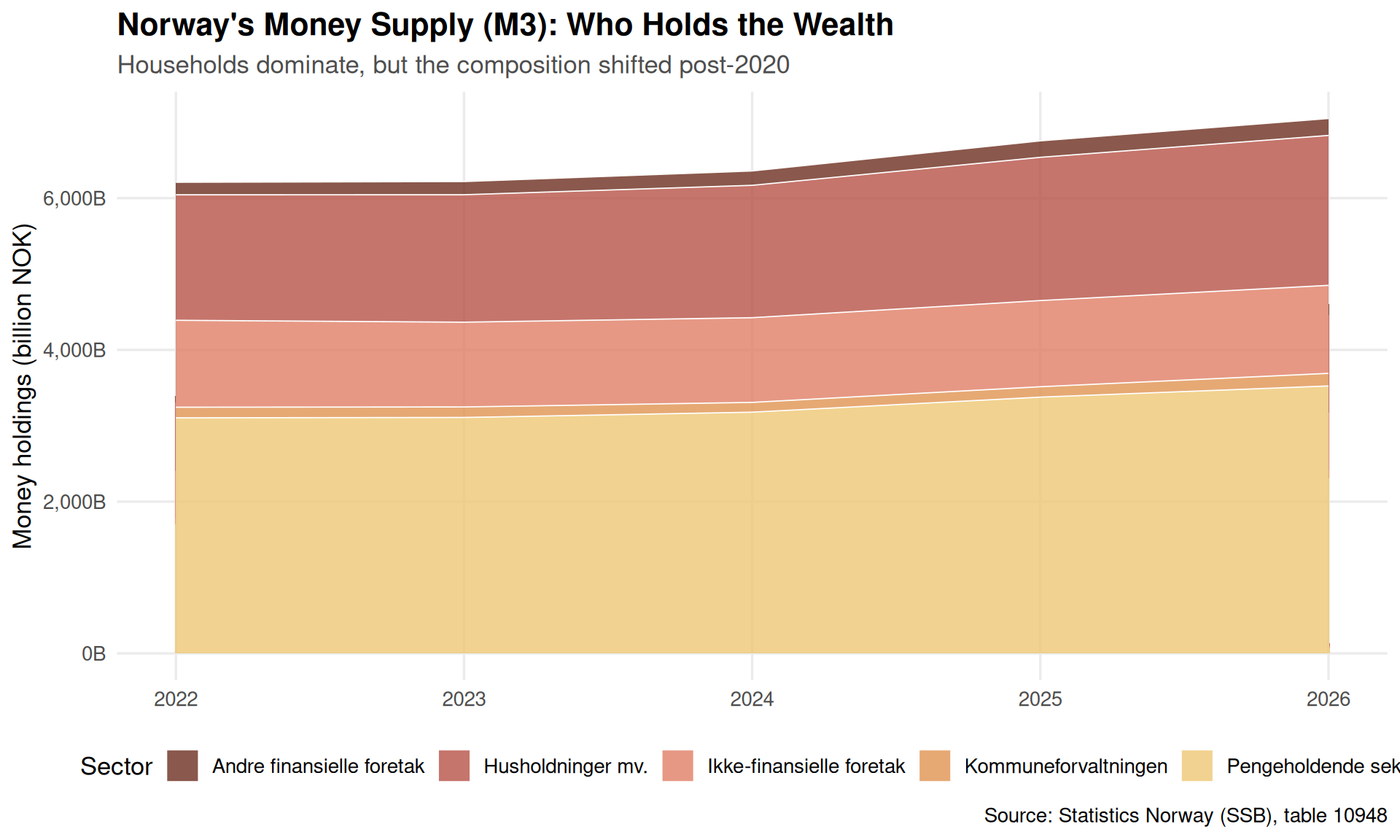
6 2023M04 3136361First, let’s see how total revenue contributions have evolved across the major economic sectors. We’ll look at the money supply measure M3 (the broadest measure of money in circulation) by sector—a proxy for economic activity and tax base.
has_monthly <- FALSE
if (!is.null(df)) {
  has_monthly <- any(stringr::str_detect(df$time_str, "M\\d{2}"), na.rm = TRUE)
  message("Data has monthly granularity: ", has_monthly)
}if (!is.null(df)) {
# Filter to M3 holdings and aggregate by sector and year
df_m3 <- df |>
filter(grepl("M3", variable, ignore.case = TRUE)) |>
group_by(year, sector) |>
summarise(value = mean(value, na.rm = TRUE), .groups = "drop") |>
filter(!is.na(value), value > 0)
if (nrow(df_m3) > 0) {
p1 <- ggplot(df_m3, aes(x = year, y = value / 1000, fill = sector)) +
geom_area(alpha = 0.8, color = "white", linewidth = 0.3) +
scale_fill_manual(values = pal) +
scale_y_continuous(labels = label_comma(suffix = "B")) +
labs(
title = "Norway's Money Supply (M3): Who Holds the Wealth",
subtitle = "Households dominate, but the composition shifted post-2020",
x = NULL,
y = "Money holdings (billion NOK)",
fill = "Sector",
caption = "Source: Statistics Norway (SSB), table 10948"
) +
theme_minimal(base_size = 13) +
theme(
legend.position = "bottom",
plot.title = element_text(face = "bold", size = 16),
plot.subtitle = element_text(color = "grey30"),
panel.grid.minor = element_blank()
)
print(p1)
}
}
How has the balance between household and corporate money holdings changed? Let’s compare the two biggest players with a slope chart.
if (!is.null(df)) {
  df_compare <- df |>
    filter(grepl("M3", variable, ignore.case = TRUE)) |>
    filter(grepl("Husholdninger|finansielle foretak", sector, ignore.case = TRUE)) |>
    group_by(year, sector) |>
    summarise(value = mean(value, na.rm = TRUE), .groups = "drop") |>
    filter(year %in% c(min(year, na.rm = TRUE), max(year, na.rm = TRUE)))

  if (nrow(df_compare) > 0) {
    p2 <- ggplot(df_compare, aes(x = factor(year), y = value / 1000, group = sector, color = sector)) +
      geom_line(linewidth = 1.5, alpha = 0.7) +
      geom_point(size = 4) +
      geom_text(
        data = df_compare |> filter(year == min(year)),
        aes(label = sector),
        hjust = 1.1, size = 3.5, fontface = "bold"
      ) +
      geom_text(
        data = df_compare |> filter(year == max(year)),
        aes(label = paste0(round(value / 1000, 0), "B")),
        hjust = -0.2, size = 3.5, fontface = "bold"
      ) +
      scale_color_manual(values = c(pal[2], pal[5])) +
      scale_y_continuous(labels = label_comma(suffix = "B")) +
      labs(
        title = "Households vs. Financial Firms: The Money Holding Gap",
        subtitle = paste0("Change from ", min(df_compare$year), " to ", max(df_compare$year)),
        x = NULL,
        y = "M3 holdings (billion NOK)",
        caption = "Source: SSB"
      ) +
      theme_minimal(base_size = 13) +
      theme(
        legend.position = "none",
        plot.title = element_text(face = "bold", size = 15),
        plot.subtitle = element_text(color = "grey30"),
        panel.grid.major.x = element_blank(),
        panel.grid.minor = element_blank()
      )
    print(p2)
  }
}
Error in `palette()`:
! Insufficient values in manual scale. 3 needed but only 2 provided.If we have monthly data, let’s see how transaction flows vary by sector throughout the year—otherwise, we’ll compare year-over-year growth rates.
if (!is.null(df) && has_monthly) {
  df_trans <- df |>
    filter(grepl("Transaksjoner siste m.ned", variable, ignore.case = TRUE)) |>
    mutate(month = month(date, label = TRUE)) |>
    filter(!is.na(month))

  if (nrow(df_trans) > 0) {
    p3 <- ggplot(df_trans, aes(x = value, y = sector, fill = sector)) +
      geom_density_ridges(alpha = 0.7, scale = 1.5) +
      scale_fill_manual(values = pal) +
      labs(
        title = "Monthly Transaction Volatility by Sector",
        subtitle = "Distribution of month-to-month changes in money supply",
        x = "Transaction volume (million NOK)",
        y = NULL,
        caption = "Source: SSB"
      ) +
      theme_minimal(base_size = 13) +
      theme(
        legend.position = "none",
        plot.title = element_text(face = "bold", size = 15),
        panel.grid.minor = element_blank()
      )
    print(p3)
  }
} else if (!is.null(df)) {
  # Annual data fallback: year-over-year growth
  df_growth <- df |>
    filter(grepl("M3", variable, ignore.case = TRUE)) |>
    arrange(sector, year) |>
    group_by(sector) |>
    mutate(yoy_pct = (value / lag(value) - 1) * 100) |>
    filter(!is.na(yoy_pct))

  if (nrow(df_growth) > 0) {
    p3 <- ggplot(df_growth, aes(x = year, y = yoy_pct, color = sector)) +
      geom_line(linewidth = 1.2) +
      geom_hline(yintercept = 0, linetype = "dashed", color = "grey50") +
      scale_color_manual(values = pal) +
      labs(
        title = "Year-Over-Year Growth in Money Holdings",
        subtitle = "Households and firms show diverging trends post-pandemic",
        x = NULL,
        y = "Annual growth (%)",
        color = "Sector",
        caption = "Source: SSB"
      ) +
      theme_minimal(base_size = 13) +
      theme(
        legend.position = "bottom",
        plot.title = element_text(face = "bold", size = 15),
        panel.grid.minor = element_blank()
      )
    print(p3)
  }
}![]()
Let’s rank sectors by their recent growth in money holdings—a dumbbell chart comparing 2020 to the latest year.
if (!is.null(df)) {
  df_dumbbell <- df |>
    filter(grepl("M3", variable, ignore.case = TRUE)) |>
    filter(year %in% c(2020, max(year, na.rm = TRUE))) |>
    group_by(sector, year) |>
    summarise(value = mean(value, na.rm = TRUE), .groups = "drop") |>
    pivot_wider(names_from = year, values_from = value, names_prefix = "y") |>
    mutate(
      change = get(paste0("y", max(df$year, na.rm = TRUE))) - y2020,
      change_pct = (change / y2020) * 100
    ) |>
    filter(!is.na(change_pct)) |>
    arrange(desc(change_pct))

  if (nrow(df_dumbbell) > 0) {
    df_dumbbell_long <- df_dumbbell |>
      pivot_longer(cols = starts_with("y"), names_to = "period", values_to = "value") |>
      mutate(period = ifelse(period == "y2020", "2020", as.character(max(df$year, na.rm = TRUE))))

    p4 <- ggplot(df_dumbbell_long, aes(x = value / 1000, y = reorder(sector, value))) +
      geom_line(aes(group = sector), color = "grey60", linewidth = 1.2) +
      geom_point(aes(color = period), size = 4) +
      scale_color_manual(values = c(pal[3], pal[6])) +
      scale_x_continuous(labels = label_comma(suffix = "B")) +
      labs(
        title = "Money Holdings: 2020 vs. 2026",
        subtitle = "Which sectors accumulated the most wealth?",
        x = "M3 holdings (billion NOK)",
        y = NULL,
        color = "Year",
        caption = "Source: SSB"
      ) +
      theme_minimal(base_size = 13) +
      theme(
        legend.position = "bottom",
        plot.title = element_text(face = "bold", size = 15),
        panel.grid.minor = element_blank()
      )
    print(p4)
  }
}
Error in `mutate()`:
ℹ In argument: `change = get(paste0("y", max(df$year, na.rm = TRUE))) -
y2020`.
Caused by error:
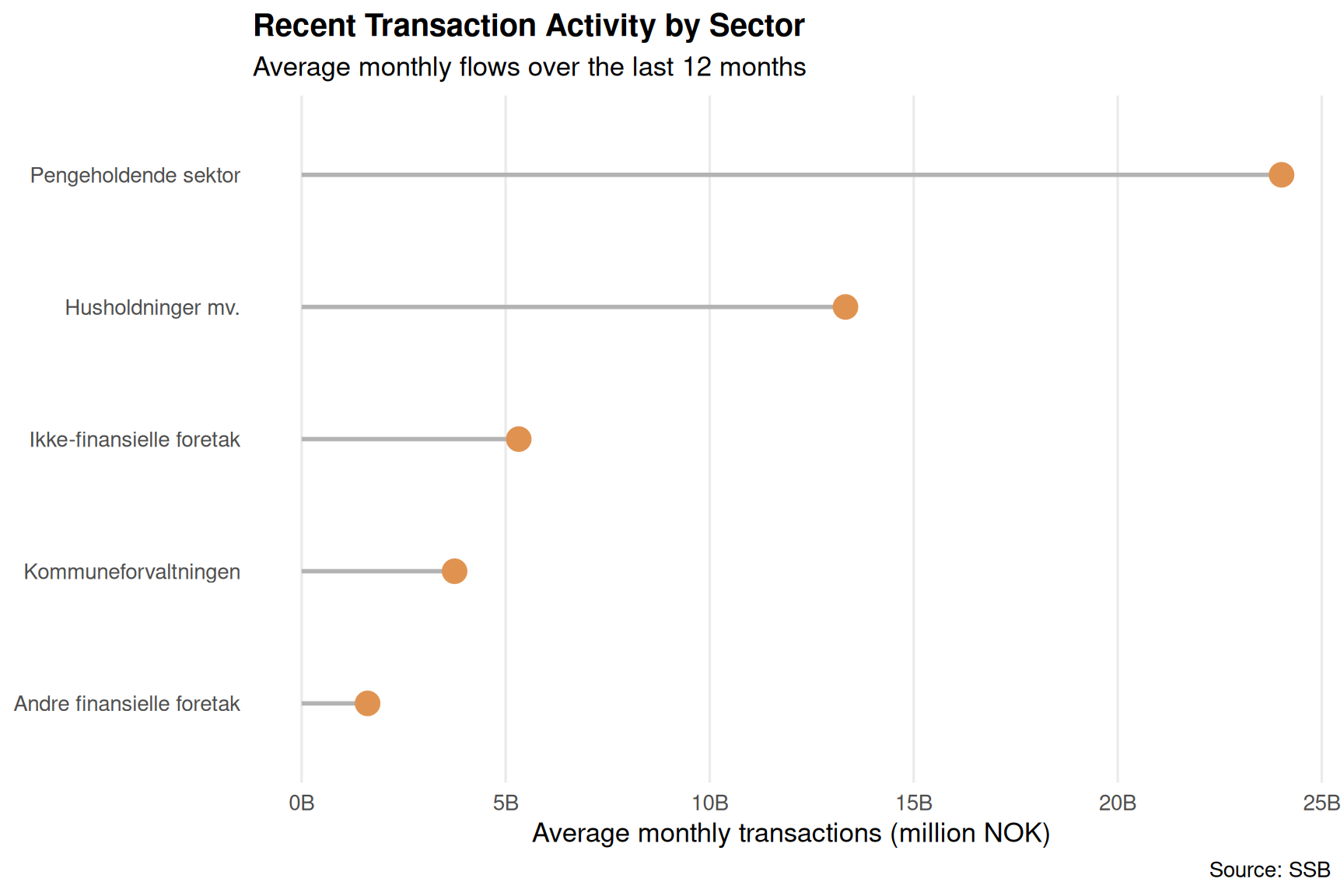
! object 'y2020' not foundFinally, let’s zoom in on the most recent period to see which sectors have driven month-to-month changes—or if we have annual data, the latest year’s performance.
if (!is.null(df)) {
  if (has_monthly) {
    df_recent <- df |>
      filter(grepl("Transaksjoner siste m.ned", variable, ignore.case = TRUE)) |>
      filter(date >= max(date, na.rm = TRUE) - months(12)) |>
      group_by(sector) |>
      summarise(avg_trans = mean(value, na.rm = TRUE), .groups = "drop") |>
      arrange(desc(avg_trans))

    ylabel <- "Average monthly transactions (million NOK)"
    title_text <- "Recent Transaction Activity by Sector"
    subtitle_text <- "Average monthly flows over the last 12 months"
  } else {
    df_recent <- df |>
      filter(grepl("M3", variable, ignore.case = TRUE)) |>
      filter(year == max(year, na.rm = TRUE)) |>
      group_by(sector) |>
      summarise(avg_trans = mean(value, na.rm = TRUE), .groups = "drop") |>
      arrange(desc(avg_trans))

    ylabel <- "Money holdings (million NOK)"
    title_text <- "Current Money Holdings by Sector"
    subtitle_text <- paste0("Latest year: ", max(df$year, na.rm = TRUE))
  }

  if (nrow(df_recent) > 0) {
    p5 <- ggplot(df_recent, aes(x = avg_trans / 1000, y = reorder(sector, avg_trans))) +
      geom_segment(
        aes(x = 0, xend = avg_trans / 1000, yend = reorder(sector, avg_trans)),
        color = "grey70",
        linewidth = 1
      ) +
      geom_point(color = pal[4], size = 5) +
      scale_x_continuous(labels = label_comma(suffix = "B")) +
      labs(
        title = title_text,
        subtitle = subtitle_text,
        x = ylabel,
        y = NULL,
        caption = "Source: SSB"
      ) +
      theme_minimal(base_size = 13) +
      theme(
        plot.title = element_text(face = "bold", size = 15),
        panel.grid.minor = element_blank(),
        panel.grid.major.y = element_blank()
      )
    print(p5)
  }
}
Norway’s fiscal base increasingly depends on household wealth and consumption taxes as corporate money holdings grow more slowly. The widening gap between household and business sector liquidity suggests that future tax policy debates will center on wealth taxation and consumption levies. Meanwhile, the municipal sector’s stable but modest money supply underscores the ongoing pressure on local government finances—a theme that connects directly to debates over property taxes and service cuts across Norwegian cities.