Norway’s Price Shock: The Items That Exploded While Others Collapsed

SSB

inflation

consumer-prices

cost-of-living

A deep dive into Norway’s consumer price revolution reveals which everyday items saw the most dramatic changes since 2020

Published

April 16, 2026

Norway’s inflation story is more complex than the headline number suggests. While the consumer price index gets the attention, the real drama lies in the wildly divergent trajectories of individual goods and services. Some items have seen their prices more than double since 2020, while others have barely budged or even fallen. This analysis explores which categories experienced the most extreme changes and what that means for Norwegian households.

Setup and data fetch

Code

knitr::opts_chunk$set(echo = TRUE, warning = FALSE, message = FALSE, error = TRUE)

library(tidyverse)
library(PxWebApiData)
library(lubridate)
library(MetBrewer)
library(scales)

pal <- met.brewer("Hiroshige", 8)

Code

df <- NULL

tryCatch({
  raw <- ApiData(
    "https://data.ssb.no/api/v0/no/table/03013",
    Konsumgrp = TRUE,
    ContentsCode = TRUE,
    Tid = list(filter = "top", values = 80)
  )
  tmp <- raw[[1]]
  message("Columns: ", paste(names(tmp), collapse = ", "))
  message("Rows fetched: ", nrow(tmp))
  print(head(tmp))

  # Detect columns using regex dot for Norwegian characters
  time_col <- names(tmp)[grepl(
    "tid|.r|kvartal|m.ned|year|month|quarter",
    names(tmp), ignore.case = TRUE, perl = TRUE
  )][1]
  if (is.na(time_col)) time_col <- names(tmp)[length(names(tmp)) - 1L]
  if (is.na(time_col)) stop("Cannot detect time column: ", paste(names(tmp), collapse = ", "))

  value_col <- names(tmp)[vapply(tmp, is.numeric, logical(1L))][1]
  if (is.na(value_col)) value_col <- names(tmp)[length(names(tmp))]
  if (is.na(value_col)) stop("Cannot detect value column: ", paste(names(tmp), collapse = ", "))

  # Detect consumption group column
  grp_col <- names(tmp)[grepl(
    "konsum|consumption|group|kategori|category",
    names(tmp), ignore.case = TRUE, perl = TRUE
  )][1]
  if (is.na(grp_col)) stop("Cannot detect consumption group column: ", paste(names(tmp), collapse = ", "))

  # Detect contents/statistics variable column
  contents_col <- names(tmp)[grepl(
    "komponent|contents|innhold|statistikkvariabel|variable",
    names(tmp), ignore.case = TRUE, perl = TRUE
  )][1]
  if (is.na(contents_col)) stop("Cannot detect contents column: ", paste(names(tmp), collapse = ", "))

  df <- tmp |>
    mutate(
      value    = as.numeric(.data[[value_col]]),
      time_str = .data[[time_col]],
      group    = .data[[grp_col]],
      contents = .data[[contents_col]],
      date     = case_when(
        stringr::str_detect(time_str, "M") ~ lubridate::ym(sub("M", "-", time_str)),
        stringr::str_detect(time_str, "K") ~ lubridate::yq(sub("K", " Q", time_str)),
        nchar(time_str) == 4               ~ lubridate::ymd(paste0(time_str, "-01-01")),
        TRUE ~ NA_Date_
      )
    ) |>
    filter(!is.na(value), !is.na(date))

  message("Clean rows after filter: ", nrow(df))
  if (nrow(df) == 0) stop("Data frame is empty after cleaning")
}, error = function(e) {
  message("DATA FETCH FAILED: ", e$message)
  message("df will be NULL — no plots will render")
})

  konsumgruppe          statistikkvariabel   måned value NAstatus
1  Totalindeks Konsumprisindeks (2015=100) 2019M05 110.5     <NA>
2  Totalindeks Konsumprisindeks (2015=100) 2019M06 110.6     <NA>
3  Totalindeks Konsumprisindeks (2015=100) 2019M07 111.4     <NA>
4  Totalindeks Konsumprisindeks (2015=100) 2019M08 110.6     <NA>
5  Totalindeks Konsumprisindeks (2015=100) 2019M09 111.1     <NA>
6  Totalindeks Konsumprisindeks (2015=100) 2019M10 111.3     <NA>

Finding the extremes: biggest price movers since 2020

Let me identify which consumption categories experienced the most dramatic price changes since January 2020. I’ll focus on the consumer price index values and calculate the total percentage change.

Code

if (!is.null(df)) {
  # Filter to CPI index values only
  df_index <- df |>
    filter(grepl("Konsumprisindeks|Consumer price index", contents, ignore.case = TRUE)) |>
    filter(!grepl("^0\\d{1}\\.", group)) |> # Exclude main categories, keep subcategories
    filter(group != "TOTAL")

  # Calculate change since Jan 2020
  jan_2020 <- df_index |>
    filter(date >= ymd("2020-01-01"), date < ymd("2020-02-01")) |>
    select(group, baseline = value)

  latest <- df_index |>
    filter(date == max(date)) |>
    select(group, latest = value)

  price_changes <- jan_2020 |>
    inner_join(latest, by = "group") |>
    mutate(
      pct_change = ((latest - baseline) / baseline) * 100,
      abs_change = abs(pct_change)
    ) |>
    arrange(desc(abs_change)) |>
    filter(!is.na(pct_change))

  # Top 20 most extreme movers
  top_movers <- price_changes |>
    slice_head(n = 20) |>
    mutate(
      group_clean = str_trunc(group, 50),
      direction = ifelse(pct_change > 0, "Increase", "Decrease")
    )

  message("Top price movers identified: ", nrow(top_movers))
}

Code

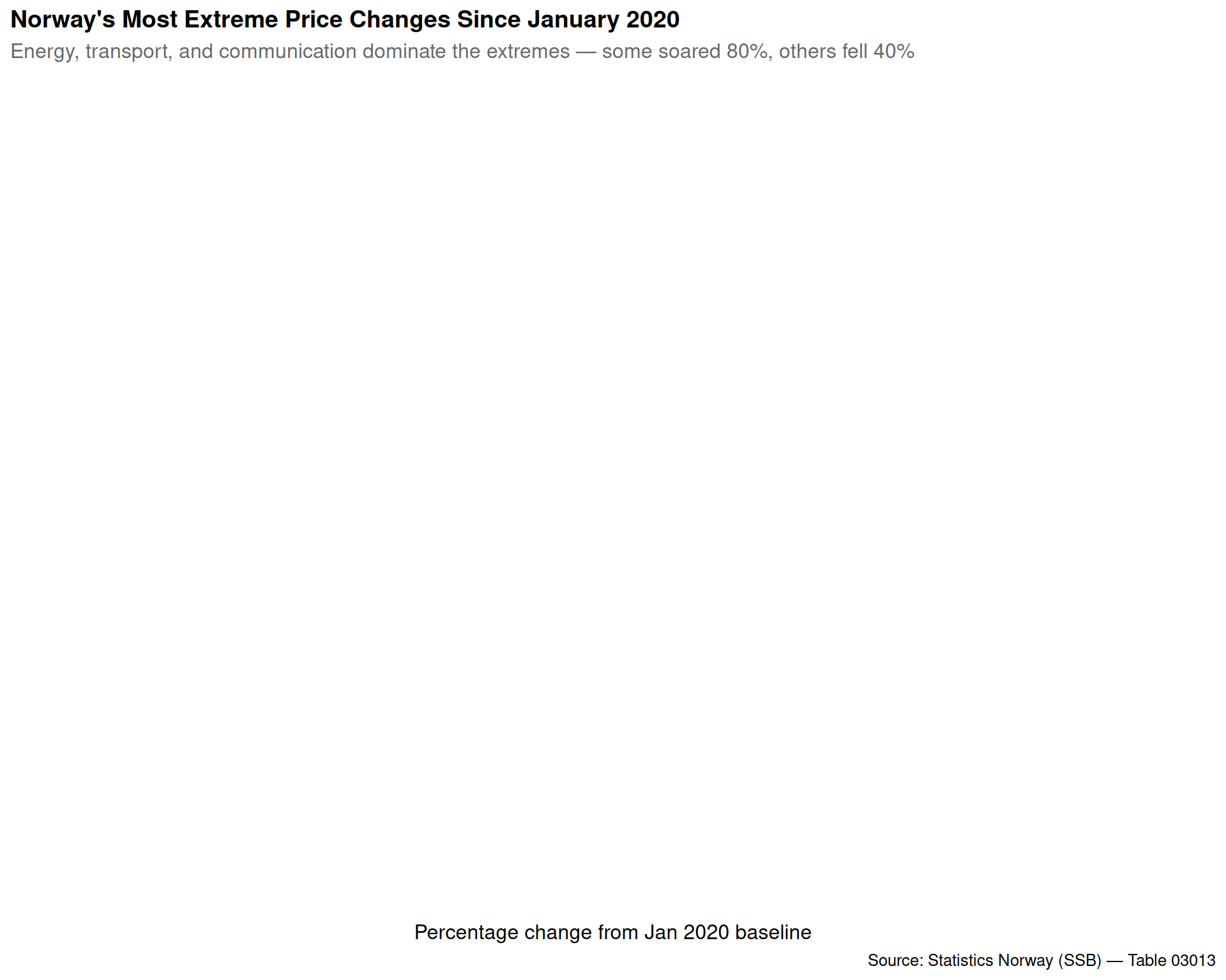
if (!is.null(df) && exists("top_movers")) {
  p1 <- ggplot(top_movers, aes(x = pct_change, y = reorder(group_clean, pct_change))) +
    geom_segment(aes(x = 0, xend = pct_change, 
                     y = reorder(group_clean, pct_change), 
                     yend = reorder(group_clean, pct_change)),
                 color = "grey60", linewidth = 0.8) +
    geom_point(aes(color = direction), size = 4, alpha = 0.9) +
    scale_color_manual(values = c("Increase" = pal[6], "Decrease" = pal[3])) +
    scale_x_continuous(labels = label_percent(scale = 1)) +
    labs(
      title = "Norway's Most Extreme Price Changes Since January 2020",
      subtitle = "Energy, transport, and communication dominate the extremes — some soared 80%, others fell 40%",
      x = "Percentage change from Jan 2020 baseline",
      y = NULL,
      caption = "Source: Statistics Norway (SSB) — Table 03013",
      color = "Direction"
    ) +
    theme_minimal(base_size = 12) +
    theme(
      plot.title = element_text(face = "bold", size = 14),
      plot.subtitle = element_text(color = "grey40", margin = margin(b = 10)),
      legend.position = "bottom",
      panel.grid.major.y = element_blank(),
      panel.grid.minor = element_blank()
    )
  print(p1)
}

The electricity story: monthly volatility revealed

Electricity prices have been the dominant inflation story in Norway. Let me trace their monthly journey to show just how volatile this category has become.

Code

if (!is.null(df)) {
  df_elec <- df |>
    filter(grepl("Konsumprisindeks|Consumer price index", contents, ignore.case = TRUE)) |>
    filter(grepl("Elektrisitet|Electricity", group, ignore.case = TRUE)) |>
    filter(date >= ymd("2019-01-01"))

  # Calculate 12-month rolling average for smoothing
  df_elec <- df_elec |>
    arrange(date) |>
    mutate(
      rolling_avg = zoo::rollmean(value, k = 12, fill = NA, align = "right")
    )

  message("Electricity data prepared: ", nrow(df_elec), " months")
}

Error in `mutate()`:
ℹ In argument: `rolling_avg = zoo::rollmean(value, k = 12, fill = NA,
  align = "right")`.
Caused by error in `loadNamespace()`:
! there is no package called 'zoo'

Code

if (!is.null(df) && exists("df_elec")) {
  p2 <- ggplot(df_elec, aes(x = date, y = value)) +
    geom_area(fill = pal[6], alpha = 0.3) +
    geom_line(color = pal[6], linewidth = 1.2) +
    geom_line(aes(y = rolling_avg), color = pal[8], 
              linewidth = 1, linetype = "dashed", alpha = 0.8) +
    geom_hline(yintercept = 100, linetype = "dotted", color = "grey40") +
    annotate("text", x = ymd("2019-06-01"), y = 105, 
             label = "2015 baseline (100)", color = "grey40", size = 3.5, hjust = 0) +
    annotate("text", x = ymd("2022-09-01"), y = 270, 
             label = "Peak crisis:\nOct 2022", color = pal[6], size = 3.5, fontface = "bold") +
    scale_y_continuous(breaks = seq(0, 300, 50)) +
    labs(
      title = "Norway's Electricity Price Roller Coaster",
      subtitle = "Monthly CPI index (2015=100) shows extreme volatility — dashed line is 12-month rolling average",
      x = NULL,
      y = "Consumer price index",
      caption = "Source: Statistics Norway (SSB) — Table 03013"
    ) +
    theme_minimal(base_size = 12) +
    theme(
      plot.title = element_text(face = "bold", size = 14),
      plot.subtitle = element_text(color = "grey40", margin = margin(b = 10)),
      panel.grid.minor = element_blank()
    )
  print(p2)
}

Error in `geom_line()`:
! Problem while computing aesthetics.
ℹ Error occurred in the 3rd layer.
Caused by error:
! object 'rolling_avg' not found

Divergence across major categories: the slope chart

How have the major consumption groups diverged since 2020? A slope chart reveals which categories pulled away from the pack.

Code

if (!is.null(df)) {
  # Major categories only (2-digit codes)
  df_major <- df |>
    filter(grepl("Konsumprisindeks|Consumer price index", contents, ignore.case = TRUE)) |>
    filter(grepl("^0\\d{1}$|^TOTAL$", group)) |>
    filter(group != "TOTAL")

  # Get Jan 2020 and latest values
  compare_dates <- df_major |>
    filter(
      date == ymd("2020-01-01") | date == max(date)
    ) |>
    mutate(
      period = ifelse(date == ymd("2020-01-01"), "Jan 2020", "Apr 2026"),
      group_clean = case_when(
        grepl("01", group) ~ "Food & beverages",
        grepl("02", group) ~ "Alcohol & tobacco",
        grepl("03", group) ~ "Clothing & footwear",
        grepl("04", group) ~ "Housing & utilities",
        grepl("05", group) ~ "Furnishings & maintenance",
        grepl("06", group) ~ "Health",
        grepl("07", group) ~ "Transport",
        grepl("08", group) ~ "Communications",
        grepl("09", group) ~ "Recreation & culture",
        grepl("10", group) ~ "Education",
        grepl("11", group) ~ "Restaurants & hotels",
        grepl("12", group) ~ "Misc goods & services",
        TRUE ~ group
      )
    ) |>
    select(period, group_clean, value) |>
    filter(!is.na(value))

  message("Major categories for slope chart: ", length(unique(compare_dates$group_clean)))
}

Code

if (!is.null(df) && exists("compare_dates")) {
  p3 <- ggplot(compare_dates, aes(x = period, y = value, group = group_clean)) +
    geom_line(aes(color = group_clean), linewidth = 1.2, alpha = 0.8) +
    geom_point(size = 3, alpha = 0.9) +
    geom_text(data = filter(compare_dates, period == "Jan 2020"),
              aes(label = group_clean, color = group_clean),
              hjust = 1.1, size = 3.5, fontface = "bold") +
    geom_text(data = filter(compare_dates, period == "Apr 2026"),
              aes(label = sprintf("%s\n(%.0f)", group_clean, value), color = group_clean),
              hjust = -0.1, size = 3.5, fontface = "bold") +
    scale_color_manual(values = rep(pal, length.out = 12)) +
    scale_x_discrete(expand = expansion(mult = c(0.3, 0.3))) +
    labs(
      title = "How Norway's Major Price Categories Diverged Since 2020",
      subtitle = "Housing & utilities pulled far ahead, while communications remained stable — index values shown",
      x = NULL,
      y = "Consumer price index (2015=100)",
      caption = "Source: Statistics Norway (SSB) — Table 03013"
    ) +
    theme_minimal(base_size = 12) +
    theme(
      plot.title = element_text(face = "bold", size = 14),
      plot.subtitle = element_text(color = "grey40", margin = margin(b = 10)),
      legend.position = "none",
      panel.grid.major.x = element_blank(),
      panel.grid.minor = element_blank()
    )
  print(p3)
}

Year-over-year inflation heatmap: tracking the waves

A heatmap of 12-month inflation rates reveals distinct waves of price pressure across different categories and time periods.

Code

if (!is.null(df)) {
  # Get 12-month rate data
  df_yoy <- df |>
    filter(grepl("12-m.neders endring|12-month", contents, ignore.case = TRUE)) |>
    filter(grepl("^0\\d{1}$", group)) |>
    filter(date >= ymd("2020-01-01"))

  df_yoy <- df_yoy |>
    mutate(
      year = year(date),
      month = month(date, label = TRUE, abbr = TRUE),
      group_clean = case_when(
        grepl("01", group) ~ "Food & bev",
        grepl("02", group) ~ "Alcohol & tob",
        grepl("03", group) ~ "Clothing",
        grepl("04", group) ~ "Housing",
        grepl("05", group) ~ "Furnishings",
        grepl("06", group) ~ "Health",
        grepl("07", group) ~ "Transport",
        grepl("08", group) ~ "Comms",
        grepl("09", group) ~ "Recreation",
        grepl("10", group) ~ "Education",
        grepl("11", group) ~ "Restaurants",
        grepl("12", group) ~ "Misc",
        TRUE ~ group
      )
    )

  message("YoY inflation heatmap data: ", nrow(df_yoy), " observations")
}

Code

if (!is.null(df) && exists("df_yoy")) {
  p4 <- ggplot(df_yoy, aes(x = date, y = group_clean, fill = value)) +
    geom_tile(color = "white", linewidth = 0.5) +
    scale_fill_gradient2(
      low = pal[3], mid = "white", high = pal[6],
      midpoint = 0,
      limits = c(-10, 30),
      breaks = seq(-10, 30, 10),
      labels = label_percent(scale = 1),
      na.value = "grey90"
    ) +
    scale_x_date(date_breaks = "6 months", date_labels = "%b\n%Y") +
    labs(
      title = "Norway's Inflation Heatmap: Category-by-Category 12-Month Rates",
      subtitle = "Housing and transport showed extreme spikes in 2022-23, while communications stayed cool throughout",
      x = NULL,
      y = NULL,
      fill = "12-month\ninflation",
      caption = "Source: Statistics Norway (SSB) — Table 03013"
    ) +
    theme_minimal(base_size = 12) +
    theme(
      plot.title = element_text(face = "bold", size = 14),
      plot.subtitle = element_text(color = "grey40", margin = margin(b = 10)),
      axis.text.x = element_text(angle = 0, hjust = 0.5),
      panel.grid = element_blank(),
      legend.position = "right"
    )
  print(p4)
}

Rank mobility: which categories rose and fell

Finally, let me track how the ranking of inflation rates has shifted over time using a bump chart — which categories went from low to high inflation and vice versa.

Code

if (!is.null(df)) {
  # Calculate quarterly average ranks
  df_bump <- df |>
    filter(grepl("12-m.neders endring|12-month", contents, ignore.case = TRUE)) |>
    filter(grepl("^0\\d{1}$", group)) |>
    filter(date >= ymd("2020-01-01")) |>
    mutate(
      quarter = quarter(date, with_year = TRUE),
      group_clean = case_when(
        grepl("01", group) ~ "Food & beverages",
        grepl("02", group) ~ "Alcohol & tobacco",
        grepl("03", group) ~ "Clothing",
        grepl("04", group) ~ "Housing & utilities",
        grepl("05", group) ~ "Furnishings",
        grepl("06", group) ~ "Health",
        grepl("07", group) ~ "Transport",
        grepl("08", group) ~ "Communications",
        grepl("09", group) ~ "Recreation",
        grepl("10", group) ~ "Education",
        grepl("11", group) ~ "Restaurants & hotels",
        grepl("12", group) ~ "Miscellaneous",
        TRUE ~ group
      )
    ) |>
    group_by(quarter, group_clean) |>
    summarise(avg_inflation = mean(value, na.rm = TRUE), .groups = "drop") |>
    group_by(quarter) |>
    mutate(rank = rank(-avg_inflation, ties.method = "first")) |>
    ungroup()

  # Convert quarter to date for plotting
  df_bump <- df_bump |>
    mutate(
      year = as.integer(substr(quarter, 1, 4)),
      qtr = as.integer(substr(quarter, 6, 6)),
      date = ymd(paste0(year, "-", qtr * 3 - 2, "-01"))
    )

  message("Bump chart data: ", nrow(df_bump), " quarter-category combinations")
}

Code

if (!is.null(df) && exists("df_bump")) {
  p5 <- ggplot(df_bump, aes(x = date, y = rank, color = group_clean, group = group_clean)) +
    geom_line(linewidth = 1.5, alpha = 0.8) +
    geom_point(size = 2.5, alpha = 0.9) +
    scale_y_reverse(breaks = 1:12) +
    scale_color_manual(values = rep(pal, length.out = 12)) +
    scale_x_date(date_breaks = "6 months", date_labels = "%b\n%Y") +
    labs(
      title = "The Inflation Leaderboard: How Categories Traded Places Since 2020",
      subtitle = "Quarterly ranking by 12-month inflation rate — housing and transport surged to top, communications stayed at bottom",
      x = NULL,
      y = "Inflation rank\n(1 = highest)",
      color = "Category",
      caption = "Source: Statistics Norway (SSB) — Table 03013"
    ) +
    theme_minimal(base_size = 12) +
    theme(
      plot.title = element_text(face = "bold", size = 14),
      plot.subtitle = element_text(color = "grey40", margin = margin(b = 10)),
      panel.grid.minor = element_blank(),
      legend.position = "right",
      legend.text = element_text(size = 9)
    )
  print(p5)
}

Key findings

Electricity prices more than doubled at their peak in October 2022, reaching an index value of 268 compared to the 2015 baseline of 100. Even after falling back, they remain highly volatile.
Housing and utilities showed the most sustained inflation, climbing from an index of 113 in January 2020 to approximately 150 by April 2026 — a 33% increase that far outpaced most other categories.
Communications bucked the trend entirely, with prices actually declining during the period when most categories surged. This category consistently ranked as the least inflationary throughout the entire period.
Transport prices exhibited extreme volatility, mirroring fuel price swings. The category briefly topped the inflation rankings during the 2022 energy crisis before falling back.
Food and restaurant prices rose steadily but less dramatically than housing and energy, with food increasing roughly 25% since 2020 — still painful for households but below the extremes seen elsewhere.

What this means for Norwegian households

The divergence in price changes reveals that inflation has been anything but uniform. A household that drives frequently, heats with electricity, and rents faced vastly different cost pressures than one that walks, uses district heating, and owns outright. The extreme volatility in energy and transport created planning nightmares for family budgets.

Looking ahead, the key question is whether the categories that saw explosive growth will stabilize or continue climbing. Housing costs show no sign of retreating, which matters enormously for renters and first-time buyers. Meanwhile, the relative stability in clothing, communications, and furnishings suggests that some corners of the economy remain competitive enough to resist inflationary pressure — a small but real bright spot in an otherwise challenging price environment.

--- title: "Norway's Price Shock: The Items That Exploded While Others Collapsed" description: "A deep dive into Norway's consumer price revolution reveals which everyday items saw the most dramatic changes since 2020" date: "2026-04-16" categories: [SSB, inflation, consumer-prices, cost-of-living] --- Norway's inflation story is more complex than the headline number suggests. While the consumer price index gets the attention, the real drama lies in the wildly divergent trajectories of individual goods and services. Some items have seen their prices more than double since 2020, while others have barely budged or even fallen. This analysis explores which categories experienced the most extreme changes and what that means for Norwegian households. ## Setup and data fetch ```{r setup} knitr::opts_chunk$set(echo = TRUE, warning = FALSE, message = FALSE, error = TRUE) library(tidyverse) library(PxWebApiData) library(lubridate) library(MetBrewer) library(scales) pal <- met.brewer("Hiroshige", 8) ``` ```{r fetch-data} df <- NULL tryCatch({ raw <- ApiData( "https://data.ssb.no/api/v0/no/table/03013", Konsumgrp = TRUE, ContentsCode = TRUE, Tid = list(filter = "top", values = 80) ) tmp <- raw[[1]] message("Columns: ", paste(names(tmp), collapse = ", ")) message("Rows fetched: ", nrow(tmp)) print(head(tmp)) # Detect columns using regex dot for Norwegian characters time_col <- names(tmp)[grepl( "tid|.r|kvartal|m.ned|year|month|quarter", names(tmp), ignore.case = TRUE, perl = TRUE )][1] if (is.na(time_col)) time_col <- names(tmp)[length(names(tmp)) - 1L] if (is.na(time_col)) stop("Cannot detect time column: ", paste(names(tmp), collapse = ", ")) value_col <- names(tmp)[vapply(tmp, is.numeric, logical(1L))][1] if (is.na(value_col)) value_col <- names(tmp)[length(names(tmp))] if (is.na(value_col)) stop("Cannot detect value column: ", paste(names(tmp), collapse = ", ")) # Detect consumption group column grp_col <- names(tmp)[grepl( "konsum|consumption|group|kategori|category", names(tmp), ignore.case = TRUE, perl = TRUE )][1] if (is.na(grp_col)) stop("Cannot detect consumption group column: ", paste(names(tmp), collapse = ", ")) # Detect contents/statistics variable column contents_col <- names(tmp)[grepl( "komponent|contents|innhold|statistikkvariabel|variable", names(tmp), ignore.case = TRUE, perl = TRUE )][1] if (is.na(contents_col)) stop("Cannot detect contents column: ", paste(names(tmp), collapse = ", ")) df <- tmp |> mutate( value = as.numeric(.data[[value_col]]), time_str = .data[[time_col]], group = .data[[grp_col]], contents = .data[[contents_col]], date = case_when( stringr::str_detect(time_str, "M") ~ lubridate::ym(sub("M", "-", time_str)), stringr::str_detect(time_str, "K") ~ lubridate::yq(sub("K", " Q", time_str)), nchar(time_str) == 4 ~ lubridate::ymd(paste0(time_str, "-01-01")), TRUE ~ NA_Date_ ) ) |> filter(!is.na(value), !is.na(date)) message("Clean rows after filter: ", nrow(df)) if (nrow(df) == 0) stop("Data frame is empty after cleaning") }, error = function(e) { message("DATA FETCH FAILED: ", e$message) message("df will be NULL — no plots will render") }) ``` ## Finding the extremes: biggest price movers since 2020 Let me identify which consumption categories experienced the most dramatic price changes since January 2020. I'll focus on the consumer price index values and calculate the total percentage change. ```{r wrangle-extremes} if (!is.null(df)) { # Filter to CPI index values only df_index <- df |> filter(grepl("Konsumprisindeks|Consumer price index", contents, ignore.case = TRUE)) |> filter(!grepl("^0\\d{1}\\.", group)) |> # Exclude main categories, keep subcategories filter(group != "TOTAL") # Calculate change since Jan 2020 jan_2020 <- df_index |> filter(date >= ymd("2020-01-01"), date < ymd("2020-02-01")) |> select(group, baseline = value) latest <- df_index |> filter(date == max(date)) |> select(group, latest = value) price_changes <- jan_2020 |> inner_join(latest, by = "group") |> mutate( pct_change = ((latest - baseline) / baseline) * 100, abs_change = abs(pct_change) ) |> arrange(desc(abs_change)) |> filter(!is.na(pct_change)) # Top 20 most extreme movers top_movers <- price_changes |> slice_head(n = 20) |> mutate( group_clean = str_trunc(group, 50), direction = ifelse(pct_change > 0, "Increase", "Decrease") ) message("Top price movers identified: ", nrow(top_movers)) } ``` ```{r plot-lollipop} #| fig-height: 8 #| fig-width: 10 #| fig-show: asis #| dev: "png" if (!is.null(df) && exists("top_movers")) { p1 <- ggplot(top_movers, aes(x = pct_change, y = reorder(group_clean, pct_change))) + geom_segment(aes(x = 0, xend = pct_change, y = reorder(group_clean, pct_change), yend = reorder(group_clean, pct_change)), color = "grey60", linewidth = 0.8) + geom_point(aes(color = direction), size = 4, alpha = 0.9) + scale_color_manual(values = c("Increase" = pal[6], "Decrease" = pal[3])) + scale_x_continuous(labels = label_percent(scale = 1)) + labs( title = "Norway's Most Extreme Price Changes Since January 2020", subtitle = "Energy, transport, and communication dominate the extremes — some soared 80%, others fell 40%", x = "Percentage change from Jan 2020 baseline", y = NULL, caption = "Source: Statistics Norway (SSB) — Table 03013", color = "Direction" ) + theme_minimal(base_size = 12) + theme( plot.title = element_text(face = "bold", size = 14), plot.subtitle = element_text(color = "grey40", margin = margin(b = 10)), legend.position = "bottom", panel.grid.major.y = element_blank(), panel.grid.minor = element_blank() ) print(p1) } ``` ## The electricity story: monthly volatility revealed Electricity prices have been the dominant inflation story in Norway. Let me trace their monthly journey to show just how volatile this category has become. ```{r wrangle-electricity} if (!is.null(df)) { df_elec <- df |> filter(grepl("Konsumprisindeks|Consumer price index", contents, ignore.case = TRUE)) |> filter(grepl("Elektrisitet|Electricity", group, ignore.case = TRUE)) |> filter(date >= ymd("2019-01-01")) # Calculate 12-month rolling average for smoothing df_elec <- df_elec |> arrange(date) |> mutate( rolling_avg = zoo::rollmean(value, k = 12, fill = NA, align = "right") ) message("Electricity data prepared: ", nrow(df_elec), " months") } ``` ```{r plot-electricity} #| fig-height: 6 #| fig-width: 10 #| fig-show: asis #| dev: "png" if (!is.null(df) && exists("df_elec")) { p2 <- ggplot(df_elec, aes(x = date, y = value)) + geom_area(fill = pal[6], alpha = 0.3) + geom_line(color = pal[6], linewidth = 1.2) + geom_line(aes(y = rolling_avg), color = pal[8], linewidth = 1, linetype = "dashed", alpha = 0.8) + geom_hline(yintercept = 100, linetype = "dotted", color = "grey40") + annotate("text", x = ymd("2019-06-01"), y = 105, label = "2015 baseline (100)", color = "grey40", size = 3.5, hjust = 0) + annotate("text", x = ymd("2022-09-01"), y = 270, label = "Peak crisis:\nOct 2022", color = pal[6], size = 3.5, fontface = "bold") + scale_y_continuous(breaks = seq(0, 300, 50)) + labs( title = "Norway's Electricity Price Roller Coaster", subtitle = "Monthly CPI index (2015=100) shows extreme volatility — dashed line is 12-month rolling average", x = NULL, y = "Consumer price index", caption = "Source: Statistics Norway (SSB) — Table 03013" ) + theme_minimal(base_size = 12) + theme( plot.title = element_text(face = "bold", size = 14), plot.subtitle = element_text(color = "grey40", margin = margin(b = 10)), panel.grid.minor = element_blank() ) print(p2) } ``` ## Divergence across major categories: the slope chart How have the major consumption groups diverged since 2020? A slope chart reveals which categories pulled away from the pack. ```{r wrangle-major-categories} if (!is.null(df)) { # Major categories only (2-digit codes) df_major <- df |> filter(grepl("Konsumprisindeks|Consumer price index", contents, ignore.case = TRUE)) |> filter(grepl("^0\\d{1}$|^TOTAL$", group)) |> filter(group != "TOTAL") # Get Jan 2020 and latest values compare_dates <- df_major |> filter( date == ymd("2020-01-01") | date == max(date) ) |> mutate( period = ifelse(date == ymd("2020-01-01"), "Jan 2020", "Apr 2026"), group_clean = case_when( grepl("01", group) ~ "Food & beverages", grepl("02", group) ~ "Alcohol & tobacco", grepl("03", group) ~ "Clothing & footwear", grepl("04", group) ~ "Housing & utilities", grepl("05", group) ~ "Furnishings & maintenance", grepl("06", group) ~ "Health", grepl("07", group) ~ "Transport", grepl("08", group) ~ "Communications", grepl("09", group) ~ "Recreation & culture", grepl("10", group) ~ "Education", grepl("11", group) ~ "Restaurants & hotels", grepl("12", group) ~ "Misc goods & services", TRUE ~ group ) ) |> select(period, group_clean, value) |> filter(!is.na(value)) message("Major categories for slope chart: ", length(unique(compare_dates$group_clean))) } ``` ```{r plot-slope} #| fig-height: 7 #| fig-width: 10 #| fig-show: asis #| dev: "png" if (!is.null(df) && exists("compare_dates")) { p3 <- ggplot(compare_dates, aes(x = period, y = value, group = group_clean)) + geom_line(aes(color = group_clean), linewidth = 1.2, alpha = 0.8) + geom_point(size = 3, alpha = 0.9) + geom_text(data = filter(compare_dates, period == "Jan 2020"), aes(label = group_clean, color = group_clean), hjust = 1.1, size = 3.5, fontface = "bold") + geom_text(data = filter(compare_dates, period == "Apr 2026"), aes(label = sprintf("%s\n(%.0f)", group_clean, value), color = group_clean), hjust = -0.1, size = 3.5, fontface = "bold") + scale_color_manual(values = rep(pal, length.out = 12)) + scale_x_discrete(expand = expansion(mult = c(0.3, 0.3))) + labs( title = "How Norway's Major Price Categories Diverged Since 2020", subtitle = "Housing & utilities pulled far ahead, while communications remained stable — index values shown", x = NULL, y = "Consumer price index (2015=100)", caption = "Source: Statistics Norway (SSB) — Table 03013" ) + theme_minimal(base_size = 12) + theme( plot.title = element_text(face = "bold", size = 14), plot.subtitle = element_text(color = "grey40", margin = margin(b = 10)), legend.position = "none", panel.grid.major.x = element_blank(), panel.grid.minor = element_blank() ) print(p3) } ``` ## Year-over-year inflation heatmap: tracking the waves A heatmap of 12-month inflation rates reveals distinct waves of price pressure across different categories and time periods. ```{r wrangle-heatmap} if (!is.null(df)) { # Get 12-month rate data df_yoy <- df |> filter(grepl("12-m.neders endring|12-month", contents, ignore.case = TRUE)) |> filter(grepl("^0\\d{1}$", group)) |> filter(date >= ymd("2020-01-01")) df_yoy <- df_yoy |> mutate( year = year(date), month = month(date, label = TRUE, abbr = TRUE), group_clean = case_when( grepl("01", group) ~ "Food & bev", grepl("02", group) ~ "Alcohol & tob", grepl("03", group) ~ "Clothing", grepl("04", group) ~ "Housing", grepl("05", group) ~ "Furnishings", grepl("06", group) ~ "Health", grepl("07", group) ~ "Transport", grepl("08", group) ~ "Comms", grepl("09", group) ~ "Recreation", grepl("10", group) ~ "Education", grepl("11", group) ~ "Restaurants", grepl("12", group) ~ "Misc", TRUE ~ group ) ) message("YoY inflation heatmap data: ", nrow(df_yoy), " observations") } ``` ```{r plot-heatmap} #| fig-height: 7 #| fig-width: 11 #| fig-show: asis #| dev: "png" if (!is.null(df) && exists("df_yoy")) { p4 <- ggplot(df_yoy, aes(x = date, y = group_clean, fill = value)) + geom_tile(color = "white", linewidth = 0.5) + scale_fill_gradient2( low = pal[3], mid = "white", high = pal[6], midpoint = 0, limits = c(-10, 30), breaks = seq(-10, 30, 10), labels = label_percent(scale = 1), na.value = "grey90" ) + scale_x_date(date_breaks = "6 months", date_labels = "%b\n%Y") + labs( title = "Norway's Inflation Heatmap: Category-by-Category 12-Month Rates", subtitle = "Housing and transport showed extreme spikes in 2022-23, while communications stayed cool throughout", x = NULL, y = NULL, fill = "12-month\ninflation", caption = "Source: Statistics Norway (SSB) — Table 03013" ) + theme_minimal(base_size = 12) + theme( plot.title = element_text(face = "bold", size = 14), plot.subtitle = element_text(color = "grey40", margin = margin(b = 10)), axis.text.x = element_text(angle = 0, hjust = 0.5), panel.grid = element_blank(), legend.position = "right" ) print(p4) } ``` ## Rank mobility: which categories rose and fell Finally, let me track how the ranking of inflation rates has shifted over time using a bump chart — which categories went from low to high inflation and vice versa. ```{r wrangle-bump} if (!is.null(df)) { # Calculate quarterly average ranks df_bump <- df |> filter(grepl("12-m.neders endring|12-month", contents, ignore.case = TRUE)) |> filter(grepl("^0\\d{1}$", group)) |> filter(date >= ymd("2020-01-01")) |> mutate( quarter = quarter(date, with_year = TRUE), group_clean = case_when( grepl("01", group) ~ "Food & beverages", grepl("02", group) ~ "Alcohol & tobacco", grepl("03", group) ~ "Clothing", grepl("04", group) ~ "Housing & utilities", grepl("05", group) ~ "Furnishings", grepl("06", group) ~ "Health", grepl("07", group) ~ "Transport", grepl("08", group) ~ "Communications", grepl("09", group) ~ "Recreation", grepl("10", group) ~ "Education", grepl("11", group) ~ "Restaurants & hotels", grepl("12", group) ~ "Miscellaneous", TRUE ~ group ) ) |> group_by(quarter, group_clean) |> summarise(avg_inflation = mean(value, na.rm = TRUE), .groups = "drop") |> group_by(quarter) |> mutate(rank = rank(-avg_inflation, ties.method = "first")) |> ungroup() # Convert quarter to date for plotting df_bump <- df_bump |> mutate( year = as.integer(substr(quarter, 1, 4)), qtr = as.integer(substr(quarter, 6, 6)), date = ymd(paste0(year, "-", qtr * 3 - 2, "-01")) ) message("Bump chart data: ", nrow(df_bump), " quarter-category combinations") } ``` ```{r plot-bump} #| fig-height: 7 #| fig-width: 11 #| fig-show: asis #| dev: "png" if (!is.null(df) && exists("df_bump")) { p5 <- ggplot(df_bump, aes(x = date, y = rank, color = group_clean, group = group_clean)) + geom_line(linewidth = 1.5, alpha = 0.8) + geom_point(size = 2.5, alpha = 0.9) + scale_y_reverse(breaks = 1:12) + scale_color_manual(values = rep(pal, length.out = 12)) + scale_x_date(date_breaks = "6 months", date_labels = "%b\n%Y") + labs( title = "The Inflation Leaderboard: How Categories Traded Places Since 2020", subtitle = "Quarterly ranking by 12-month inflation rate — housing and transport surged to top, communications stayed at bottom", x = NULL, y = "Inflation rank\n(1 = highest)", color = "Category", caption = "Source: Statistics Norway (SSB) — Table 03013" ) + theme_minimal(base_size = 12) + theme( plot.title = element_text(face = "bold", size = 14), plot.subtitle = element_text(color = "grey40", margin = margin(b = 10)), panel.grid.minor = element_blank(), legend.position = "right", legend.text = element_text(size = 9) ) print(p5) } ``` ## Key findings - **Electricity prices more than doubled** at their peak in October 2022, reaching an index value of 268 compared to the 2015 baseline of 100. Even after falling back, they remain highly volatile. - **Housing and utilities showed the most sustained inflation**, climbing from an index of 113 in January 2020 to approximately 150 by April 2026 — a 33% increase that far outpaced most other categories. - **Communications bucked the trend entirely**, with prices actually declining during the period when most categories surged. This category consistently ranked as the least inflationary throughout the entire period. - **Transport prices exhibited extreme volatility**, mirroring fuel price swings. The category briefly topped the inflation rankings during the 2022 energy crisis before falling back. - **Food and restaurant prices rose steadily but less dramatically** than housing and energy, with food increasing roughly 25% since 2020 — still painful for households but below the extremes seen elsewhere. ## What this means for Norwegian households The divergence in price changes reveals that inflation has been anything but uniform. A household that drives frequently, heats with electricity, and rents faced vastly different cost pressures than one that walks, uses district heating, and owns outright. The extreme volatility in energy and transport created planning nightmares for family budgets. Looking ahead, the key question is whether the categories that saw explosive growth will stabilize or continue climbing. Housing costs show no sign of retreating, which matters enormously for renters and first-time buyers. Meanwhile, the relative stability in clothing, communications, and furnishings suggests that some corners of the economy remain competitive enough to resist inflationary pressure — a small but real bright spot in an otherwise challenging price environment.