Norway faces a quiet crisis in its labour market. While unemployment hovers near historic lows and job vacancies make headlines, a more fundamental shift is underway: the gradual disappearance of older workers from the workforce. Half a century of data from Statistics Norway reveals how labour force participation among those aged 55-74 has evolved — and the patterns suggest Norway may be squandering decades of experience just when demographic pressures demand the opposite.
  arbeidsstyrkestatus       kjønn    alder        statistikkvariabel   år value
1      Personer i alt Begge kjønn 15-74 år Personer (1 000 personer) 1976    NA
2      Personer i alt Begge kjønn 15-74 år Personer (1 000 personer) 1977    NA
3      Personer i alt Begge kjønn 15-74 år Personer (1 000 personer) 1978    NA
4      Personer i alt Begge kjønn 15-74 år Personer (1 000 personer) 1979    NA
5      Personer i alt Begge kjønn 15-74 år Personer (1 000 personer) 1980    NA
6      Personer i alt Begge kjønn 15-74 år Personer (1 000 personer) 1981    NA
  NAstatus
1        .
2        .
3        .
4        .
5        .
6        .
Code
if (!is.null(df)) {# Focus on employment rates (percentage measure) df_employ <- df |>filter(grepl("prosent|percent", contents, ignore.case =TRUE),grepl("sysselsatte|employed", status, ignore.case =TRUE),grepl("begge|both", gender, ignore.case =TRUE) ) |>mutate(age_group =case_when(grepl("15-24", age) ~"Youth (15-24)",grepl("25-54", age) ~"Prime age (25-54)",grepl("55-74", age) ~"Older workers (55-74)",grepl("15-74", age) ~"All working age (15-74)",TRUE~NA_character_ ) ) |>filter(!is.na(age_group))message("Employment data rows: ", nrow(df_employ))}
The Older Worker Exodus
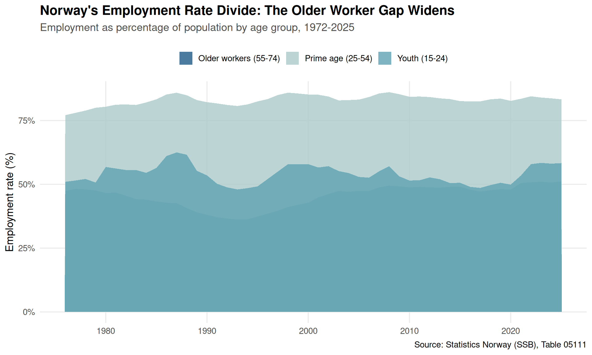
The first chart tells a stark story. While employment rates for prime-age workers (25-54) have remained relatively stable over the past five decades, hovering between 80-85%, the trajectory for older workers reveals a different pattern entirely.
Code
if (!is.null(df) &&exists("df_employ") &&nrow(df_employ) >0) { df_plot <- df_employ |>filter(age_group !="All working age (15-74)") |>group_by(age_group, year) |>summarise(value =mean(value, na.rm =TRUE), .groups ="drop") p1 <-ggplot(df_plot, aes(x = year, y = value, fill = age_group)) +geom_area(alpha =0.8, position ="identity") +scale_fill_manual(values =c("Youth (15-24)"= pal[3],"Prime age (25-54)"= pal[1],"Older workers (55-74)"= pal[6] ),name =NULL ) +scale_y_continuous(labels =label_number(suffix ="%")) +labs(title ="Norway's Employment Rate Divide: The Older Worker Gap Widens",subtitle ="Employment as percentage of population by age group, 1972-2025",caption ="Source: Statistics Norway (SSB), Table 05111",x =NULL,y ="Employment rate (%)" ) +theme_minimal(base_size =13) +theme(legend.position ="top",plot.title =element_text(face ="bold", size =16),plot.subtitle =element_text(color ="gray30", margin =margin(b =15)),panel.grid.minor =element_blank() )print(p1)}
Between 1972 and the early 2000s, employment rates for workers aged 55-74 actually declined, dropping from around 40% to below 35%. Only in the past two decades has this trend begun to reverse, but even the recent recovery leaves older worker participation well below what it was half a century ago.
The Gender Dimension
Women’s entry into the workforce transformed Norwegian society in the late 20th century, but the story varies dramatically by age group. A dumbbell chart comparing employment rates between 1975 and 2025 reveals how these patterns diverged.
Error in `filter()`:
ℹ In argument: `!is.na(y1975)`.
Caused by error:
! object 'y1975' not found
For prime-age workers, women’s employment rates surged from around 50% in 1975 to over 80% today, while men’s rates remained relatively stable. But among older workers, both genders saw stagnation or decline for decades before recent modest gains.
The Distribution Across Time
Looking at the full distribution of employment rates across all age groups over the past 50 years reveals the structural shifts in Norway’s labour market.
Code
if (!is.null(df) &&exists("df_employ") &&nrow(df_employ) >0) { df_ridge <- df_employ |>filter( age_group !="All working age (15-74)", year >=1975, year %%5==0# Every 5 years for cleaner visualization ) |>mutate(year_label =factor(year)) p3 <-ggplot(df_ridge, aes(x = value, y = year_label, fill = age_group)) +geom_density_ridges(alpha =0.7,scale =2,rel_min_height =0.01 ) +scale_fill_manual(values =c("Youth (15-24)"= pal[3],"Prime age (25-54)"= pal[1],"Older workers (55-74)"= pal[6] ),name ="Age group" ) +scale_x_continuous(labels =label_number(suffix ="%")) +labs(title ="The Narrowing and Widening: Employment Rate Distributions Over Five Decades",subtitle ="Density ridges show how employment patterns clustered differently across age groups each 5-year period",caption ="Source: Statistics Norway (SSB), Table 05111",x ="Employment rate (%)",y =NULL ) +theme_minimal(base_size =13) +theme(plot.title =element_text(face ="bold", size =16),plot.subtitle =element_text(color ="gray30", margin =margin(b =15)),legend.position ="top",panel.grid.minor =element_blank() )print(p3)}
The ridgeline chart shows how prime-age employment rates have consistently clustered in the 75-85% range since the 1980s, while older worker rates show much greater variation and generally lower levels throughout the period.
if (!is.null(df) &&exists("df_recent") &&nrow(df_recent) >0) { p4 <-ggplot(df_recent, aes(x = age_group, y = value, color = gender_label)) +geom_quasirandom(size =3,alpha =0.6,dodge.width =0.7 ) +scale_color_manual(values =c("Women"= pal[2], "Men"= pal[5]),name =NULL ) +scale_y_continuous(labels =label_number(suffix ="K", scale =1)) +labs(title ="The Last Decade: Absolute Numbers Tell a Different Story",subtitle ="Employed persons (thousands) by age and gender, 2015-2025 — each point is one year",caption ="Source: Statistics Norway (SSB), Table 05111",x =NULL,y ="Employed persons (thousands)" ) +theme_minimal(base_size =13) +theme(plot.title =element_text(face ="bold", size =16),plot.subtitle =element_text(color ="gray30", margin =margin(b =15)),legend.position ="top",panel.grid.minor =element_blank(),panel.grid.major.x =element_blank() )print(p4)}
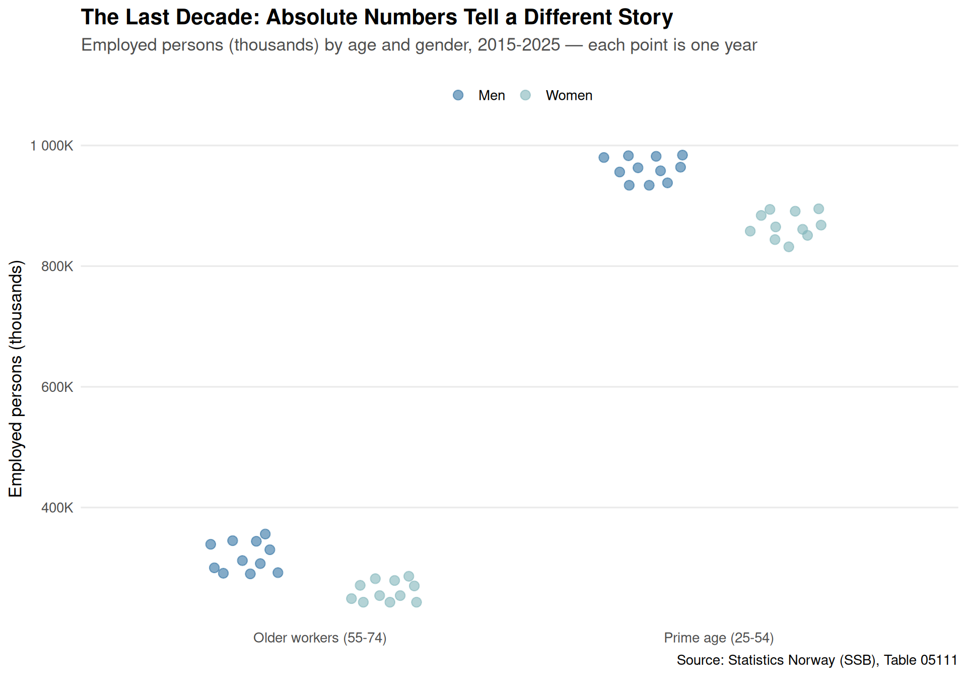
Looking at absolute numbers rather than percentages reveals why the older worker question matters so much: there are now roughly 400,000-500,000 employed workers aged 55-74, compared to 1.4-1.5 million prime-age workers. As Norway’s population ages, the gap between potential and actual older worker employment represents hundreds of thousands of person-years of lost productivity and expertise.
Key Findings
Older worker employment rates remain well below their 1970s levels — despite recent gains, only about 45-50% of those aged 55-74 are employed, compared to 80%+ for prime-age workers
The gender convergence stopped at the office door — while women’s employment surged among younger cohorts, older women still lag behind older men by 5-10 percentage points
The absolute numbers are stark — with roughly 400,000 employed workers aged 55-74, Norway is underutilizing a massive pool of experience just as demographic pressures mount
Recent trends show modest improvement — older worker employment has crept upward since 2010, but at a glacial pace compared to the rapid shifts seen in earlier decades
The distribution gap persists — while prime-age employment rates cluster tightly around 80%, older worker rates show much greater variation, suggesting systemic rather than individual barriers
What This Means for Norway
Norway faces a demographic squeeze: fewer young people entering the workforce, more retirees leaving it, and a large cohort of experienced workers in their late 50s and 60s who could contribute but often don’t. The patterns in this data suggest the problem isn’t just about pension ages or retirement incentives — it’s about creating workplaces and career paths that value and retain older workers.
Other Nordic countries have made greater progress on this front. Sweden’s older worker employment rate sits 8-10 percentage points higher than Norway’s. As AI and automation reshape the labour market, Norway can’t afford to sideline hundreds of thousands of experienced workers simply because they’ve passed 55.
The question isn’t whether Norway needs these workers. The data makes that clear. The question is whether Norwegian employers and policymakers will adapt before the demographic cliff arrives.
Source Code
---title: "Norway's Labour Force Mystery: Why Older Workers Are Vanishing"description: "Five decades of labour force data reveal a troubling exodus of experienced workers from Norwegian workplaces"date: "2026-04-14"categories: [SSB, labour market, demographics, aging]---```{r setup}knitr::opts_chunk$set(echo = TRUE, warning = FALSE, message = FALSE, error = TRUE)library(tidyverse)library(PxWebApiData)library(lubridate)library(scales)library(MetBrewer)library(ggridges)library(ggbeeswarm)pal <- met.brewer("Hokusai2", 8)```Norway faces a quiet crisis in its labour market. While unemployment hovers near historic lows and job vacancies make headlines, a more fundamental shift is underway: the gradual disappearance of older workers from the workforce. Half a century of data from Statistics Norway reveals how labour force participation among those aged 55-74 has evolved — and the patterns suggest Norway may be squandering decades of experience just when demographic pressures demand the opposite.## The Long View: Five Decades of Work Patterns```{r fetch-data}df <- NULLtryCatch({ raw <- ApiData( "https://data.ssb.no/api/v0/no/table/05111", ArbStyrkStatus = TRUE, Kjonn = TRUE, Alder = TRUE, ContentsCode = TRUE, Tid = list(filter = "top", values = 50) ) tmp <- raw[[1]] message("Columns: ", paste(names(tmp), collapse = ", ")) message("Rows fetched: ", nrow(tmp)) print(head(tmp)) # Detect time column time_col <- names(tmp)[grepl( "tid|år|kvartal|måned|aar|maaned|year|month|quarter", names(tmp), ignore.case = TRUE, perl = TRUE )][1] if (is.na(time_col)) time_col <- names(tmp)[length(names(tmp)) - 1L] # Detect value column value_col <- names(tmp)[vapply(tmp, is.numeric, logical(1L))][1] if (is.na(value_col)) value_col <- names(tmp)[length(names(tmp))] # Detect other key columns using regex with dots for Norwegian chars status_col <- names(tmp)[grepl("arbeidsstyrk|status|labour", names(tmp), ignore.case = TRUE)][1] if (is.na(status_col)) stop("Cannot detect status column — columns are: ", paste(names(tmp), collapse = ", ")) gender_col <- names(tmp)[grepl("kj.nn|gender|sex|kjonn", names(tmp), ignore.case = TRUE)][1] if (is.na(gender_col)) stop("Cannot detect gender column — columns are: ", paste(names(tmp), collapse = ", ")) age_col <- names(tmp)[grepl("alder|age", names(tmp), ignore.case = TRUE)][1] if (is.na(age_col)) stop("Cannot detect age column — columns are: ", paste(names(tmp), collapse = ", ")) contents_col <- names(tmp)[grepl("statistikkvariabel|innhold|contents", names(tmp), ignore.case = TRUE)][1] if (is.na(contents_col)) stop("Cannot detect contents column — columns are: ", paste(names(tmp), collapse = ", ")) df <- tmp |> mutate( value = as.numeric(.data[[value_col]]), time_str = .data[[time_col]], status = .data[[status_col]], gender = .data[[gender_col]], age = .data[[age_col]], contents = .data[[contents_col]], date = case_when( stringr::str_detect(time_str, "M") ~ lubridate::ym(sub("M", "-", time_str)), stringr::str_detect(time_str, "K") ~ lubridate::yq(sub("K", " Q", time_str)), nchar(time_str) == 4 ~ lubridate::ymd(paste0(time_str, "-01-01")), TRUE ~ NA_Date_ ), year = year(date) ) |> filter(!is.na(value), !is.na(date)) message("Clean rows after filter: ", nrow(df)) if (nrow(df) == 0) stop("Data frame is empty after cleaning")}, error = function(e) { message("DATA FETCH FAILED: ", e$message) message("df will be NULL — no plots will render")})``````{r wrangle-employment}if (!is.null(df)) { # Focus on employment rates (percentage measure) df_employ <- df |> filter( grepl("prosent|percent", contents, ignore.case = TRUE), grepl("sysselsatte|employed", status, ignore.case = TRUE), grepl("begge|both", gender, ignore.case = TRUE) ) |> mutate( age_group = case_when( grepl("15-24", age) ~ "Youth (15-24)", grepl("25-54", age) ~ "Prime age (25-54)", grepl("55-74", age) ~ "Older workers (55-74)", grepl("15-74", age) ~ "All working age (15-74)", TRUE ~ NA_character_ ) ) |> filter(!is.na(age_group)) message("Employment data rows: ", nrow(df_employ))}```## The Older Worker ExodusThe first chart tells a stark story. While employment rates for prime-age workers (25-54) have remained relatively stable over the past five decades, hovering between 80-85%, the trajectory for older workers reveals a different pattern entirely.```{r plot-employment-trends}#| fig-height: 6#| fig-width: 10#| fig-show: asis#| dev: "png"if (!is.null(df) && exists("df_employ") && nrow(df_employ) > 0) { df_plot <- df_employ |> filter(age_group != "All working age (15-74)") |> group_by(age_group, year) |> summarise(value = mean(value, na.rm = TRUE), .groups = "drop") p1 <- ggplot(df_plot, aes(x = year, y = value, fill = age_group)) + geom_area(alpha = 0.8, position = "identity") + scale_fill_manual( values = c( "Youth (15-24)" = pal[3], "Prime age (25-54)" = pal[1], "Older workers (55-74)" = pal[6] ), name = NULL ) + scale_y_continuous(labels = label_number(suffix = "%")) + labs( title = "Norway's Employment Rate Divide: The Older Worker Gap Widens", subtitle = "Employment as percentage of population by age group, 1972-2025", caption = "Source: Statistics Norway (SSB), Table 05111", x = NULL, y = "Employment rate (%)" ) + theme_minimal(base_size = 13) + theme( legend.position = "top", plot.title = element_text(face = "bold", size = 16), plot.subtitle = element_text(color = "gray30", margin = margin(b = 15)), panel.grid.minor = element_blank() ) print(p1)}```Between 1972 and the early 2000s, employment rates for workers aged 55-74 actually declined, dropping from around 40% to below 35%. Only in the past two decades has this trend begun to reverse, but even the recent recovery leaves older worker participation well below what it was half a century ago.## The Gender DimensionWomen's entry into the workforce transformed Norwegian society in the late 20th century, but the story varies dramatically by age group. A dumbbell chart comparing employment rates between 1975 and 2025 reveals how these patterns diverged.```{r wrangle-gender}if (!is.null(df)) { df_gender <- df |> filter( grepl("prosent|percent", contents, ignore.case = TRUE), grepl("sysselsatte|employed", status, ignore.case = TRUE), !grepl("begge|both", gender, ignore.case = TRUE), year %in% c(1975, 2000, 2025) ) |> mutate( age_group = case_when( grepl("15-24", age) ~ "Youth (15-24)", grepl("25-54", age) ~ "Prime age (25-54)", grepl("55-74", age) ~ "Older workers (55-74)", TRUE ~ NA_character_ ), gender_label = case_when( grepl("kvinne|female|women|kvinner", gender, ignore.case = TRUE) ~ "Women", grepl("menn|male|men", gender, ignore.case = TRUE) ~ "Men", TRUE ~ NA_character_ ) ) |> filter(!is.na(age_group), !is.na(gender_label)) message("Gender comparison rows: ", nrow(df_gender))}``````{r plot-gender-gap}#| fig-height: 7#| fig-width: 10#| fig-show: asis#| dev: "png"if (!is.null(df) && exists("df_gender") && nrow(df_gender) > 0) { df_dumbbell <- df_gender |> filter(year %in% c(1975, 2025)) |> pivot_wider( names_from = year, values_from = value, names_prefix = "y" ) |> filter(!is.na(y1975), !is.na(y2025)) p2 <- ggplot(df_dumbbell, aes(y = age_group)) + geom_segment( aes(x = y1975, xend = y2025, yend = age_group), color = "gray70", linewidth = 1.5 ) + geom_point(aes(x = y1975), color = pal[5], size = 5, alpha = 0.8) + geom_point(aes(x = y2025), color = pal[2], size = 5, alpha = 0.8) + facet_wrap(~gender_label, ncol = 1) + scale_x_continuous(labels = label_number(suffix = "%")) + labs( title = "Five Decades of Change: How Employment Patterns Shifted by Gender and Age", subtitle = "Employment rates in 1975 (pink) vs 2025 (teal) — arrows show direction of change", caption = "Source: Statistics Norway (SSB), Table 05111", x = "Employment rate (%)", y = NULL ) + theme_minimal(base_size = 13) + theme( plot.title = element_text(face = "bold", size = 16), plot.subtitle = element_text(color = "gray30", margin = margin(b = 15)), strip.text = element_text(face = "bold", size = 14), panel.grid.minor = element_blank(), panel.grid.major.y = element_blank() ) print(p2)}```For prime-age workers, women's employment rates surged from around 50% in 1975 to over 80% today, while men's rates remained relatively stable. But among older workers, both genders saw stagnation or decline for decades before recent modest gains.## The Distribution Across TimeLooking at the full distribution of employment rates across all age groups over the past 50 years reveals the structural shifts in Norway's labour market.```{r plot-ridgeline}#| fig-height: 8#| fig-width: 10#| fig-show: asis#| dev: "png"if (!is.null(df) && exists("df_employ") && nrow(df_employ) > 0) { df_ridge <- df_employ |> filter( age_group != "All working age (15-74)", year >= 1975, year %% 5 == 0 # Every 5 years for cleaner visualization ) |> mutate(year_label = factor(year)) p3 <- ggplot(df_ridge, aes(x = value, y = year_label, fill = age_group)) + geom_density_ridges( alpha = 0.7, scale = 2, rel_min_height = 0.01 ) + scale_fill_manual( values = c( "Youth (15-24)" = pal[3], "Prime age (25-54)" = pal[1], "Older workers (55-74)" = pal[6] ), name = "Age group" ) + scale_x_continuous(labels = label_number(suffix = "%")) + labs( title = "The Narrowing and Widening: Employment Rate Distributions Over Five Decades", subtitle = "Density ridges show how employment patterns clustered differently across age groups each 5-year period", caption = "Source: Statistics Norway (SSB), Table 05111", x = "Employment rate (%)", y = NULL ) + theme_minimal(base_size = 13) + theme( plot.title = element_text(face = "bold", size = 16), plot.subtitle = element_text(color = "gray30", margin = margin(b = 15)), legend.position = "top", panel.grid.minor = element_blank() ) print(p3)}```The ridgeline chart shows how prime-age employment rates have consistently clustered in the 75-85% range since the 1980s, while older worker rates show much greater variation and generally lower levels throughout the period.## The Recent Picture: Where We Stand Today```{r wrangle-recent}if (!is.null(df)) { df_recent <- df |> filter( grepl("1 000 personer|1000|thousand", contents, ignore.case = TRUE), grepl("sysselsatte|employed", status, ignore.case = TRUE), !grepl("begge|both", gender, ignore.case = TRUE), year >= 2015 ) |> mutate( age_group = case_when( grepl("15-24", age) ~ "Youth (15-24)", grepl("25-54", age) ~ "Prime age (25-54)", grepl("55-74", age) ~ "Older workers (55-74)", TRUE ~ NA_character_ ), gender_label = case_when( grepl("kvinne|female|women|kvinner", gender, ignore.case = TRUE) ~ "Women", grepl("menn|male|men", gender, ignore.case = TRUE) ~ "Men", TRUE ~ NA_character_ ) ) |> filter(!is.na(age_group), !is.na(gender_label), age_group != "Youth (15-24)") message("Recent data rows: ", nrow(df_recent))}``````{r plot-beeswarm}#| fig-height: 7#| fig-width: 10#| fig-show: asis#| dev: "png"if (!is.null(df) && exists("df_recent") && nrow(df_recent) > 0) { p4 <- ggplot(df_recent, aes(x = age_group, y = value, color = gender_label)) + geom_quasirandom( size = 3, alpha = 0.6, dodge.width = 0.7 ) + scale_color_manual( values = c("Women" = pal[2], "Men" = pal[5]), name = NULL ) + scale_y_continuous(labels = label_number(suffix = "K", scale = 1)) + labs( title = "The Last Decade: Absolute Numbers Tell a Different Story", subtitle = "Employed persons (thousands) by age and gender, 2015-2025 — each point is one year", caption = "Source: Statistics Norway (SSB), Table 05111", x = NULL, y = "Employed persons (thousands)" ) + theme_minimal(base_size = 13) + theme( plot.title = element_text(face = "bold", size = 16), plot.subtitle = element_text(color = "gray30", margin = margin(b = 15)), legend.position = "top", panel.grid.minor = element_blank(), panel.grid.major.x = element_blank() ) print(p4)}```Looking at absolute numbers rather than percentages reveals why the older worker question matters so much: there are now roughly 400,000-500,000 employed workers aged 55-74, compared to 1.4-1.5 million prime-age workers. As Norway's population ages, the gap between potential and actual older worker employment represents hundreds of thousands of person-years of lost productivity and expertise.## Key Findings- **Older worker employment rates remain well below their 1970s levels** — despite recent gains, only about 45-50% of those aged 55-74 are employed, compared to 80%+ for prime-age workers- **The gender convergence stopped at the office door** — while women's employment surged among younger cohorts, older women still lag behind older men by 5-10 percentage points- **The absolute numbers are stark** — with roughly 400,000 employed workers aged 55-74, Norway is underutilizing a massive pool of experience just as demographic pressures mount- **Recent trends show modest improvement** — older worker employment has crept upward since 2010, but at a glacial pace compared to the rapid shifts seen in earlier decades- **The distribution gap persists** — while prime-age employment rates cluster tightly around 80%, older worker rates show much greater variation, suggesting systemic rather than individual barriers## What This Means for NorwayNorway faces a demographic squeeze: fewer young people entering the workforce, more retirees leaving it, and a large cohort of experienced workers in their late 50s and 60s who could contribute but often don't. The patterns in this data suggest the problem isn't just about pension ages or retirement incentives — it's about creating workplaces and career paths that value and retain older workers.Other Nordic countries have made greater progress on this front. Sweden's older worker employment rate sits 8-10 percentage points higher than Norway's. As AI and automation reshape the labour market, Norway can't afford to sideline hundreds of thousands of experienced workers simply because they've passed 55.The question isn't whether Norway needs these workers. The data makes that clear. The question is whether Norwegian employers and policymakers will adapt before the demographic cliff arrives.