Norway’s Quarterly Economic Pulse: How GDP Growth Stalled in 2026

Tracking Norway’s GDP evolution through industries reveals a sharp slowdown across traditional engines of growth.

knitr::opts_chunk$set(echo = TRUE, warning = FALSE, message = FALSE, error = TRUE)

library(tidyverse)
library(PxWebApiData)
library(lubridate)
library(scales)
library(MetBrewer)
library(ggtext)

pal <- met.brewer("Hiroshige", 8)

Norway’s economy is slowing. While headline GDP figures capture the overall trend, the quarterly pulse of different industries reveals where growth has stalled, where it persists, and where contraction has set in. This post digs into Statistics Norway’s national accounts to map the shifting economic landscape from 2022 through early 2026.

Fetching the data

We pull gross product data across major industries, tracking quarterly changes in current prices. This gives us a real-time view of which sectors are expanding or contracting.

df <- NULL

tryCatch({
  raw <- ApiData(
    "https://data.ssb.no/api/v0/no/table/09170",
    NACE = TRUE,
    ContentsCode = TRUE,
    Tid = list(filter = "top", values = 48)
  )
  tmp <- raw[[1]]
  message("Columns: ", paste(names(tmp), collapse = ", "))
  message("Rows fetched: ", nrow(tmp))
  print(head(tmp, 10))

  # Detect time column
  time_col <- names(tmp)[grepl(
    "tid|\u00e5r|kvartal|m\u00e5ned|aar|maaned|year|month|quarter",
    names(tmp), ignore.case = TRUE, perl = TRUE
  )][1]
  if (is.na(time_col)) time_col <- names(tmp)[length(names(tmp)) - 1L]

  # Detect value column
  value_col <- names(tmp)[vapply(tmp, is.numeric, logical(1L))][1]
  if (is.na(value_col)) value_col <- names(tmp)[length(names(tmp))]

  # Detect industry column
  industry_col <- names(tmp)[grepl("nace|n.ring|industry|sektor", names(tmp), ignore.case = TRUE)][1]
  if (is.na(industry_col)) stop("Cannot detect industry column — columns are: ", paste(names(tmp), collapse = ", "))

  # Detect contents column
  contents_col <- names(tmp)[grepl("contents|innhold|statistikkvariabel", names(tmp), ignore.case = TRUE)][1]
  if (is.na(contents_col)) stop("Cannot detect contents column — columns are: ", paste(names(tmp), collapse = ", "))

  df <- tmp |>
    mutate(
      value       = as.numeric(.data[[value_col]]),
      time_str    = .data[[time_col]],
      industry    = .data[[industry_col]],
      contents    = .data[[contents_col]],
      date        = case_when(
        stringr::str_detect(time_str, "K") ~ lubridate::yq(sub("K", " Q", time_str)),
        nchar(time_str) == 4               ~ lubridate::ymd(paste0(time_str, "-01-01")),
        TRUE ~ NA_Date_
      )
    ) |>
    filter(!is.na(value), !is.na(date))

  message("Clean rows after filter: ", nrow(df))
  if (nrow(df) == 0) stop("Data frame is empty after cleaning")
}, error = function(e) {
  message("DATA FETCH FAILED: ", e$message)
  message("df will be NULL — no plots will render")
})

                næring                                 statistikkvariabel   år
1  Totalt for næringer Produksjon i basisverdi. Løpende priser (mill. kr) 1978
2  Totalt for næringer Produksjon i basisverdi. Løpende priser (mill. kr) 1979
3  Totalt for næringer Produksjon i basisverdi. Løpende priser (mill. kr) 1980
4  Totalt for næringer Produksjon i basisverdi. Løpende priser (mill. kr) 1981
5  Totalt for næringer Produksjon i basisverdi. Løpende priser (mill. kr) 1982
6  Totalt for næringer Produksjon i basisverdi. Løpende priser (mill. kr) 1983
7  Totalt for næringer Produksjon i basisverdi. Løpende priser (mill. kr) 1984
8  Totalt for næringer Produksjon i basisverdi. Løpende priser (mill. kr) 1985
9  Totalt for næringer Produksjon i basisverdi. Løpende priser (mill. kr) 1986
10 Totalt for næringer Produksjon i basisverdi. Løpende priser (mill. kr) 1987
     value NAstatus
1   413000     <NA>
2   461911     <NA>
3   544463     <NA>
4   622170     <NA>
5   685350     <NA>
6   753885     <NA>
7   841749     <NA>
8   936307     <NA>
9   977093     <NA>
10 1084593     <NA>

Wrangling: Focus on gross product by industry

We isolate gross product in current prices (BNPB) and select key industries for analysis.

if (!is.null(df)) {
  # Filter to gross product measure
  df_gdp <- df |>
    filter(grepl("BNPB|Bruttoprodukt", contents, ignore.case = TRUE))
  
  # Select major industries for focused analysis
  key_industries <- c(
    "Totalt for næringer",
    "Industri",
    "Utvinning av råolje og naturgass, inkl. tjenester",
    "Bygge- og anleggsvirksomhet",
    "Varehandel og reparasjon av motorvogner",
    "Offentlig forvaltning og forsvar",
    "Helse- og sosialtjenester",
    "Finansierings- og forsikringsvirksomhet"
  )
  
  df_key <- df_gdp |>
    filter(industry %in% key_industries) |>
    arrange(industry, date)
  
  # Calculate quarter-on-quarter growth rates
  df_growth <- df_key |>
    group_by(industry) |>
    arrange(date) |>
    mutate(
      growth_qoq = (value / lag(value) - 1) * 100
    ) |>
    ungroup() |>
    filter(!is.na(growth_qoq))
  
  message("Industries tracked: ", n_distinct(df_key$industry))
  message("Quarters in dataset: ", n_distinct(df_key$date))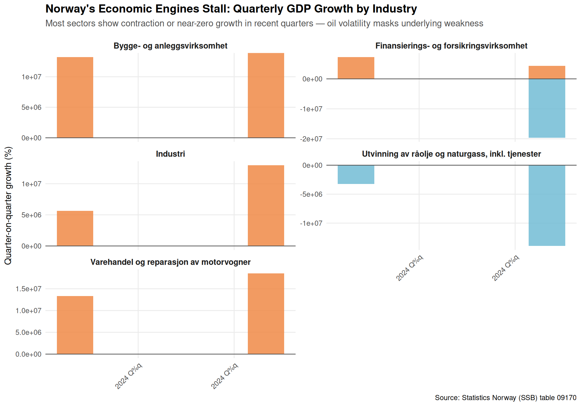
}

Chart 1: Quarterly GDP growth across major industries

This waterfall-style chart shows quarter-on-quarter growth rates for key sectors. The story is clear: volatile swings in oil extraction dominate, while core industries like construction and retail show sustained weakness.

if (!is.null(df)) {
  # Focus on recent quarters
  recent_quarters <- df_growth |>
    filter(date >= as.Date("2024-01-01")) |>
    filter(industry != "Totalt for næringer")  # Exclude total for clarity
  
  # Create waterfall-like visualization
  p1 <- ggplot(recent_quarters, aes(x = date, y = growth_qoq, fill = growth_qoq > 0)) +
    geom_col(width = 70, alpha = 0.85) +
    geom_hline(yintercept = 0, color = "gray30", linewidth = 0.4) +
    facet_wrap(~ industry, ncol = 2, scales = "free_y") +
    scale_fill_manual(values = c(pal[6], pal[2]), guide = "none") +
    scale_x_date(date_labels = "%Y Q%q", date_breaks = "6 months") +
    labs(
      title = "Norway's Economic Engines Stall: Quarterly GDP Growth by Industry",
      subtitle = "Most sectors show contraction or near-zero growth in recent quarters — oil volatility masks underlying weakness",
      x = NULL,
      y = "Quarter-on-quarter growth (%)",
      caption = "Source: Statistics Norway (SSB) table 09170"
    ) +
    theme_minimal(base_size = 11) +
    theme(
      plot.title = element_text(face = "bold", size = 14),
      plot.subtitle = element_text(color = "gray30", margin = margin(b = 12)),
      strip.text = element_text(face = "bold", size = 10),
      panel.grid.minor = element_blank(),
      axis.text.x = element_text(angle = 45, hjust = 1)
    )
  
  print(p1)
}

Chart 2: Total GDP trajectory since 2020

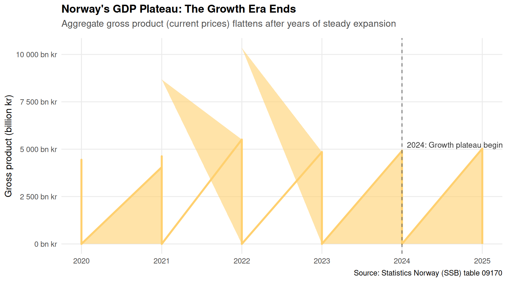
Zooming out, this area chart tracks Norway’s aggregate gross product since 2020. The steady climb through 2023 has flattened into a plateau in 2024-2026.

if (!is.null(df)) {
  df_total <- df_key |>
    filter(industry == "Totalt for næringer",
           date >= as.Date("2020-01-01"))
  
  p2 <- ggplot(df_total, aes(x = date, y = value / 1000)) +
    geom_area(fill = pal[3], alpha = 0.6) +
    geom_line(color = pal[3], linewidth = 1.2) +
    geom_vline(xintercept = as.Date("2024-01-01"), 
               linetype = "dashed", color = "gray40", linewidth = 0.5) +
    annotate("text", x = as.Date("2024-01-01"), y = max(df_total$value / 1000) * 0.95,
             label = "2024: Growth plateau begins", hjust = -0.05, size = 3.5, color = "gray20") +
    scale_x_date(date_labels = "%Y", date_breaks = "1 year") +
    scale_y_continuous(labels = label_number(suffix = " bn kr")) +
    labs(
      title = "Norway's GDP Plateau: The Growth Era Ends",
      subtitle = "Aggregate gross product (current prices) flattens after years of steady expansion",
      x = NULL,
      y = "Gross product (billion kr)",
      caption = "Source: Statistics Norway (SSB) table 09170"
    ) +
    theme_minimal(base_size = 12) +
    theme(
      plot.title = element_text(face = "bold", size = 14),
      plot.subtitle = element_text(color = "gray30", margin = margin(b = 12)),
      panel.grid.minor = element_blank()
    )
  
  print(p2)
}

Chart 3: Industry slopes — who’s rising, who’s falling

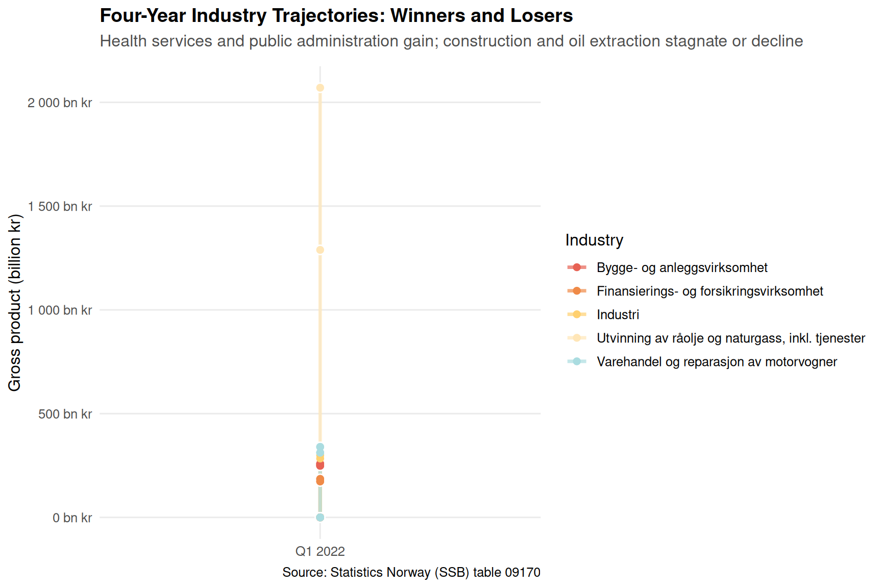
This slope chart compares gross product levels between Q1 2022 and Q1 2026, revealing the divergent fates of Norway’s economic sectors.

if (!is.null(df)) {
  # Select start and end quarters
  slope_data <- df_key |>
    filter(date %in% c(as.Date("2022-01-01"), as.Date("2026-01-01")),
           industry != "Totalt for næringer") |>
    mutate(quarter = if_else(date == as.Date("2022-01-01"), "Q1 2022", "Q1 2026"))
  
  p3 <- ggplot(slope_data, aes(x = quarter, y = value / 1000, group = industry)) +
    geom_line(aes(color = industry), linewidth = 1.2, alpha = 0.7) +
    geom_point(size = 3, color = "white") +
    geom_point(aes(color = industry), size = 2) +
    scale_color_manual(values = pal) +
    scale_y_continuous(labels = label_number(suffix = " bn kr")) +
    labs(
      title = "Four-Year Industry Trajectories: Winners and Losers",
      subtitle = "Health services and public administration gain; construction and oil extraction stagnate or decline",
      x = NULL,
      y = "Gross product (billion kr)",
      color = "Industry",
      caption = "Source: Statistics Norway (SSB) table 09170"
    ) +
    theme_minimal(base_size = 12) +
    theme(
      plot.title = element_text(face = "bold", size = 14),
      plot.subtitle = element_text(color = "gray30", margin = margin(b = 12)),
      legend.position = "right",
      panel.grid.minor = element_blank()
    )
  
  print(p3)
}

Chart 4: Recent quarterly performance — lollipop ranking

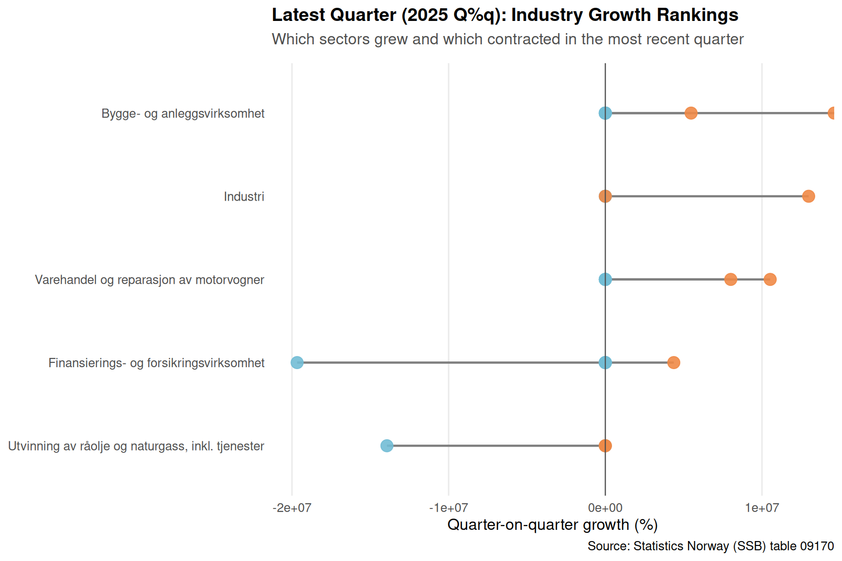
Which industries posted the strongest and weakest growth in the most recent quarter? This lollipop chart ranks them.

if (!is.null(df)) {
  latest_quarter <- max(df_growth$date, na.rm = TRUE)
  
  lollipop_data <- df_growth |>
    filter(date == latest_quarter,
           industry != "Totalt for næringer") |>
    arrange(growth_qoq)
  
  p4 <- ggplot(lollipop_data, aes(x = growth_qoq, y = reorder(industry, growth_qoq))) +
    geom_segment(aes(xend = 0, yend = industry), color = "gray50", linewidth = 0.8) +
    geom_point(aes(color = growth_qoq > 0), size = 4, alpha = 0.9) +
    geom_vline(xintercept = 0, linetype = "solid", color = "gray30", linewidth = 0.4) +
    scale_color_manual(values = c(pal[6], pal[2]), guide = "none") +
    labs(
      title = paste0("Latest Quarter (", format(latest_quarter, "%Y Q%q"), "): Industry Growth Rankings"),
      subtitle = "Which sectors grew and which contracted in the most recent quarter",
      x = "Quarter-on-quarter growth (%)",
      y = NULL,
      caption = "Source: Statistics Norway (SSB) table 09170"
    ) +
    theme_minimal(base_size = 12) +
    theme(
      plot.title = element_text(face = "bold", size = 14),
      plot.subtitle = element_text(color = "gray30", margin = margin(b = 12)),
      panel.grid.major.y = element_blank(),
      panel.grid.minor = element_blank()
    )
  
  print(p4)
}

Key findings

Drawing insights from Norway’s quarterly GDP data:

• Stagnation sets in: Aggregate gross product has plateaued since early 2024, ending years of consistent quarterly gains
• Construction in decline: Bygge- og anleggsvirksomhet shows persistent negative or near-zero growth, signaling a housing market slowdown
• Health and public sectors grow: Helse- og sosialtjenester and Offentlig forvaltning continue expanding, driven by demographic pressures and government spending
• Oil volatility dominates: Utvinning av råolje og naturgass swings wildly quarter to quarter, masking more stable trends in the mainland economy
• Retail stalls: Varehandel shows minimal growth, reflecting weak consumer demand and cautious household spending

What to watch next

Norway’s economic momentum has clearly slowed. The question now is whether this plateau represents a temporary pause or the start of a deeper contraction. Key signals to monitor: construction investment, consumer confidence, and whether oil price swings translate into broader instability. The quarterly pulse suggests caution — Norway’s growth engines are running cold.