Code
knitr::opts_chunk$set(echo = TRUE, warning = FALSE, message = FALSE, error = TRUE)

library(tidyverse)
library(PxWebApiData)
library(lubridate)
library(scales)
library(MetBrewer)

pal <- met.brewer("Hokusai1", 7)Norway has witnessed one of the most dramatic crime declines in the developed world, yet the story beneath the headline numbers reveals a complex transformation. While property crimes have plummeted, other categories tell different stories — some rising, others stubbornly persistent. This analysis examines three decades of police-reported offences to understand what’s really happening on Norwegian streets.
knitr::opts_chunk$set(echo = TRUE, warning = FALSE, message = FALSE, error = TRUE)
library(tidyverse)
library(PxWebApiData)
library(lubridate)
library(scales)
library(MetBrewer)
pal <- met.brewer("Hokusai1", 7)df <- NULL
tryCatch({
raw <- ApiData(
"https://data.ssb.no/api/v0/no/table/08484",
LovbruddKrim = TRUE,
ContentsCode = TRUE,
Tid = list(filter = "top", values = 32)
)
tmp <- raw[[1]]
message("Columns: ", paste(names(tmp), collapse = ", "))
message("Rows fetched: ", nrow(tmp))
print(head(tmp, 10))
# Detect time column
time_col <- names(tmp)[grepl(
"tid|\u00e5r|kvartal|m\u00e5ned|aar|maaned|year|month|quarter",
names(tmp), ignore.case = TRUE, perl = TRUE
)][1]
if (is.na(time_col)) time_col <- names(tmp)[length(names(tmp)) - 1L]
# Detect value column
value_col <- names(tmp)[vapply(tmp, is.numeric, logical(1L))][1]
if (is.na(value_col)) value_col <- names(tmp)[length(names(tmp))]
# Detect crime type column
crime_col <- names(tmp)[grepl("lovbrudd|offence|crime", names(tmp), ignore.case = TRUE)][1]
if (is.na(crime_col)) stop("Cannot detect crime column — columns are: ", paste(names(tmp), collapse = ", "))
# Detect contents/statistic type column
contents_col <- names(tmp)[grepl("statistikkvariabel|contents|innhold|komponent", names(tmp), ignore.case = TRUE)][1]
if (is.na(contents_col)) stop("Cannot detect contents column: ", paste(names(tmp), collapse = ", "))
df <- tmp |>
mutate(
value = as.numeric(.data[[value_col]]),
time_str = .data[[time_col]],
crime_type = .data[[crime_col]],
stat_type = .data[[contents_col]],
date = case_when(
stringr::str_detect(time_str, "M") ~ lubridate::ym(sub("M", "-", time_str)),
stringr::str_detect(time_str, "K") ~ lubridate::yq(sub("K", " Q", time_str)),
nchar(time_str) == 4 ~ lubridate::ymd(paste0(time_str, "-01-01")),
TRUE ~ NA_Date_
),
year = year(date)
) |>
filter(!is.na(value), !is.na(date))
message("Clean rows after filter: ", nrow(df))
if (nrow(df) == 0) stop("Data frame is empty after cleaning")
}, error = function(e) {
message("DATA FETCH FAILED: ", e$message)
message("df will be NULL — no plots will render")
}) lovbruddstype statistikkvariabel år value NAstatus
1 Alle lovbruddsgrupper Lovbrudd anmeldt 1993 NA .
2 Alle lovbruddsgrupper Lovbrudd anmeldt 1994 NA .
3 Alle lovbruddsgrupper Lovbrudd anmeldt 1995 NA .
4 Alle lovbruddsgrupper Lovbrudd anmeldt 1996 NA .
5 Alle lovbruddsgrupper Lovbrudd anmeldt 1997 NA .
6 Alle lovbruddsgrupper Lovbrudd anmeldt 1998 NA .
7 Alle lovbruddsgrupper Lovbrudd anmeldt 1999 NA .
8 Alle lovbruddsgrupper Lovbrudd anmeldt 2000 NA .
9 Alle lovbruddsgrupper Lovbrudd anmeldt 2001 NA .
10 Alle lovbruddsgrupper Lovbrudd anmeldt 2002 NA .Let’s start with the broadest view — total reported offences across all categories. The scale of the transformation becomes immediately clear.
if (!is.null(df)) {

  total_df <- df |>
    filter(
      grepl("Alle lovbruddsgrupper|All", crime_type, ignore.case = TRUE),
      grepl("Lovbrudd anmeldt|reported", stat_type, ignore.case = TRUE)
    ) |>
    arrange(date)

  if (nrow(total_df) > 0) {
    peak_year <- total_df |> filter(value == max(value)) |> pull(year) |> first()
    peak_value <- max(total_df$value)
    recent_value <- total_df |> filter(year == max(year)) |> pull(value) |> first()

    p1 <- ggplot(total_df, aes(x = date, y = value)) +
      geom_area(fill = pal[1], alpha = 0.7) +
      geom_line(color = pal[7], linewidth = 1) +
      annotate("text", x = as.Date("2002-01-01"), y = peak_value - 10000,
               label = paste0("Peak: ", comma(peak_year), "\n", comma(round(peak_value/1000, 0)), "k offences"),
               family = "sans", size = 3.5, hjust = 0) +
      annotate("segment", x = as.Date("2004-01-01"), xend = as.Date(paste0(peak_year, "-01-01")),
               y = peak_value - 15000, yend = peak_value - 5000,
               arrow = arrow(length = unit(0.2, "cm")), color = pal[7]) +
      scale_y_continuous(labels = comma_format()) +
      labs(
        title = "Norway's Crime Collapse: Total Reported Offences Since 1993",
        subtitle = paste0("From ", comma(round(peak_value/1000, 0)), "k offences at peak to ",
                         comma(round(recent_value/1000, 0)), "k today — a ",
                         round((1 - recent_value/peak_value)*100, 0), "% decline"),
        caption = "Source: Statistics Norway (SSB) | Table 08484",
        x = NULL,
        y = "Reported offences"
      ) +
      theme_minimal(base_size = 12) +
      theme(
        plot.title = element_text(face = "bold", size = 14),
        plot.subtitle = element_text(color = "gray40", size = 11),
        panel.grid.minor = element_blank()
      )

    print(p1)
  }
}
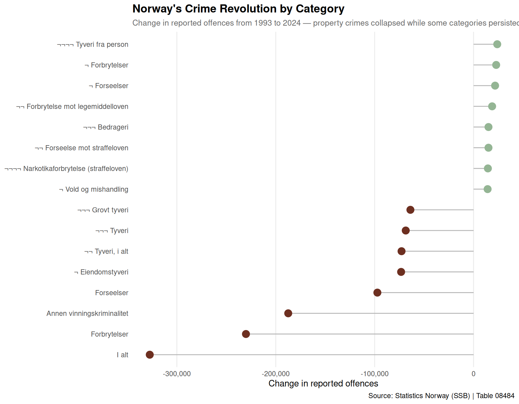
Not all crime categories have followed the same trajectory. Let’s examine which categories have seen the largest absolute changes between the earliest and most recent years available.
if (!is.null(df)) {

  category_df <- df |>
    filter(
      grepl("Lovbrudd anmeldt|reported", stat_type, ignore.case = TRUE),
      !grepl("Alle lovbruddsgrupper|All|total", crime_type, ignore.case = TRUE)
    ) |>
    group_by(crime_type) |>
    filter(n() >= 20) |>  # Only categories with substantial data
    arrange(date) |>
    mutate(
      first_value = first(value),
      last_value = last(value),
      change = last_value - first_value,
      pct_change = (last_value - first_value) / first_value * 100
    ) |>
    ungroup() |>
    distinct(crime_type, first_value, last_value, change, pct_change)

  if (nrow(category_df) > 0) {

    # Clean up crime type names - extract descriptive part
    category_df <- category_df |>
      mutate(
        crime_clean = str_remove(crime_type, "^[0-9A-Z]+AAAA-[0-9A-Z]+ZZZZz ¬+ "),
        crime_clean = str_remove(crime_clean, "^[0-9A-Z]+[A-Z][a-z]+ ¬+ "),
        crime_clean = str_trim(crime_clean)
      ) |>
      filter(nchar(crime_clean) > 3, abs(change) > 1000) |>
      arrange(change) |>
      slice(c(1:8, (n()-7):n()))  # Top and bottom 8

    p2 <- ggplot(category_df, aes(x = change, y = reorder(crime_clean, change))) +
      geom_segment(aes(x = 0, xend = change, y = crime_clean, yend = crime_clean),
                   color = "gray70", linewidth = 0.5) +
      geom_point(aes(color = change > 0), size = 4, show.legend = FALSE) +
      scale_color_manual(values = c("TRUE" = pal[6], "FALSE" = pal[1])) +
      scale_x_continuous(labels = comma_format()) +
      labs(
        title = "Norway's Crime Revolution by Category",
        subtitle = "Change in reported offences from 1993 to 2024 — property crimes collapsed while some categories persisted",
        caption = "Source: Statistics Norway (SSB) | Table 08484",
        x = "Change in reported offences",
        y = NULL
      ) +
      theme_minimal(base_size = 11) +
      theme(
        plot.title = element_text(face = "bold", size = 14),
        plot.subtitle = element_text(color = "gray40", size = 10),
        panel.grid.major.y = element_blank(),
        panel.grid.minor = element_blank()
      )

    print(p2)
  }
}
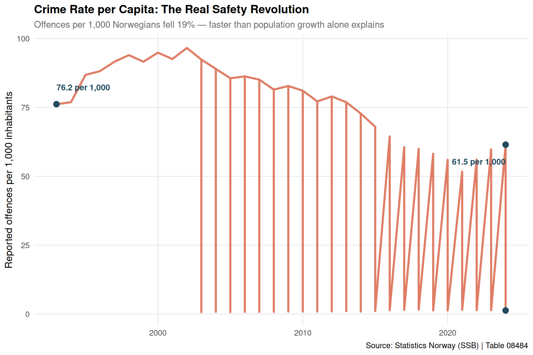
Crime rates per 1,000 inhabitants tell a different story than raw numbers — accounting for population growth reveals whether society is actually becoming safer or just growing faster than crime.
if (!is.null(df)) {

  per_capita_df <- df |>
    filter(
      grepl("Alle lovbruddsgrupper|All", crime_type, ignore.case = TRUE),
      grepl("per 1000|per capita", stat_type, ignore.case = TRUE)
    ) |>
    arrange(date)

  if (nrow(per_capita_df) > 0) {

    first_rate <- per_capita_df |> filter(year == min(year)) |> pull(value) |> first()
    last_rate <- per_capita_df |> filter(year == max(year)) |> pull(value) |> first()

    p3 <- ggplot(per_capita_df, aes(x = date, y = value)) +
      geom_line(color = pal[3], linewidth = 1.2) +
      geom_point(data = per_capita_df |> filter(year %in% c(min(year), max(year))),
                 color = pal[7], size = 3) +
      annotate("text",
               x = per_capita_df |> filter(year == min(year)) |> pull(date) |> first(),
               y = first_rate + 5,
               label = paste0(round(first_rate, 1), " per 1,000"),
               hjust = 0, vjust = 0, size = 3.5, color = pal[7], fontface = "bold") +
      annotate("text",
               x = per_capita_df |> filter(year == max(year)) |> pull(date) |> first(),
               y = last_rate - 5,
               label = paste0(round(last_rate, 1), " per 1,000"),
               hjust = 1, vjust = 1, size = 3.5, color = pal[7], fontface = "bold") +
      scale_y_continuous(labels = comma_format()) +
      labs(
        title = "Crime Rate per Capita: The Real Safety Revolution",
        subtitle = paste0("Offences per 1,000 Norwegians fell ", round((1 - last_rate/first_rate)*100, 0),
                         "% — faster than population growth alone explains"),
        caption = "Source: Statistics Norway (SSB) | Table 08484",
        x = NULL,
        y = "Reported offences per 1,000 inhabitants"
      ) +
      theme_minimal(base_size = 12) +
      theme(
        plot.title = element_text(face = "bold", size = 14),
        plot.subtitle = element_text(color = "gray40", size = 11),
        panel.grid.minor = element_blank()
      )

    print(p3)
  }
}
A heatmap view of major crime categories over the past decade reveals which offence types remain volatile and which have stabilized at lower levels.
if (!is.null(df)) {

  heatmap_df <- df |>
    filter(
      grepl("Lovbrudd anmeldt|reported", stat_type, ignore.case = TRUE),
      !grepl("Alle lovbruddsgrupper|All|total", crime_type, ignore.case = TRUE),
      year >= 2014
    ) |>
    mutate(
      crime_clean = str_remove(crime_type, "^[0-9A-Z]+AAAA-[0-9A-Z]+ZZZZz ¬+ "),
      crime_clean = str_remove(crime_clean, "^[0-9A-Z]+[A-Z][a-z]+ ¬+ "),
      crime_clean = str_trim(crime_clean)
    ) |>
    filter(nchar(crime_clean) > 3) |>
    group_by(crime_clean) |>
    filter(n() >= 8) |>  # Ensure consistent data
    mutate(scaled_value = scale(value)[,1]) |>  # Z-score standardization
    ungroup()

  if (nrow(heatmap_df) > 0) {

    # Select most variable categories
    top_categories <- heatmap_df |>
      group_by(crime_clean) |>
      summarise(variability = sd(value, na.rm = TRUE)) |>
      arrange(desc(variability)) |>
      slice(1:15) |>
      pull(crime_clean)

    heatmap_df <- heatmap_df |>
      filter(crime_clean %in% top_categories)

    p4 <- ggplot(heatmap_df, aes(x = year, y = reorder(crime_clean, scaled_value), fill = scaled_value)) +
      geom_tile(color = "white", linewidth = 0.5) +
      scale_fill_gradientn(
        colors = c(pal[1], "white", pal[6]),
        name = "Standardized\noffence rate",
        labels = c("Low", "Average", "High")
      ) +
      scale_x_continuous(breaks = seq(2014, 2024, 2)) +
      labs(
        title = "Crime Category Volatility: The Last Decade",
        subtitle = "Standardized offence rates show which crime types remain most variable year-to-year",
        caption = "Source: Statistics Norway (SSB) | Table 08484 | Colors show z-scores",
        x = NULL,
        y = NULL
      ) +
      theme_minimal(base_size = 11) +
      theme(
        plot.title = element_text(face = "bold", size = 14),
        plot.subtitle = element_text(color = "gray40", size = 10),
        legend.position = "right",
        panel.grid = element_blank(),
        axis.text.y = element_text(size = 9)
      )

    print(p4)
  }
}
Error in `scale_fill_gradientn()`:
! `breaks` and `labels` have different lengths.Based on three decades of police-reported crime data:
The Norwegian crime collapse reflects multiple converging forces: improved security technology (alarms, cameras, vehicle immobilizers), demographic shifts (aging population), economic development, and potentially changing reporting behaviors. The dramatic fall in property crimes suggests target-hardening measures worked — stolen cars and burgled homes became rarer as technology made them harder to steal and easier to trace.
But the story isn’t uniform. Drug offences and certain fraud categories remain stubborn or have grown, reflecting new challenges in a digital age. The next decade will test whether crime stabilizes at these historically low levels or whether new forms of offending — particularly cyber-enabled crimes — begin to drive numbers upward again. For now, Norway stands as one of the world’s safest societies by conventional crime measures, a remarkable achievement that has unfolded quietly over thirty years.