Code
knitr::opts_chunk$set(echo = TRUE, warning = FALSE, message = FALSE, error = TRUE)

library(tidyverse)
library(PxWebApiData)
library(lubridate)
library(MetBrewer)
library(scales)

pal <- met.brewer("Hokusai2", 8)knitr::opts_chunk$set(echo = TRUE, warning = FALSE, message = FALSE, error = TRUE)
library(tidyverse)
library(PxWebApiData)
library(lubridate)
library(MetBrewer)
library(scales)
pal <- met.brewer("Hokusai2", 8)Norway’s job vacancy rate has become one of the most watched economic indicators since the pandemic. While unemployment figures grab headlines, vacancy data tells us where the economy is actually expanding or contracting — industry by industry, quarter by quarter. The latest figures reveal a stark bifurcation: some sectors are desperately hiring while others have gone into deep freeze.
df <- NULL

tryCatch({
  raw <- ApiData(
    "https://data.ssb.no/api/v0/no/table/08771",
    NACE2007 = TRUE,
    ContentsCode = TRUE,
    Tid = list(filter = "top", values = 60)
  )
  tmp <- raw[[1]]
  message("Columns: ", paste(names(tmp), collapse = ", "))
  message("Rows fetched: ", nrow(tmp))
  print(head(tmp))

  time_col <- names(tmp)[grepl(
    "tid|år|kvartal|måned|aar|maaned|year|month|quarter",
    names(tmp), ignore.case = TRUE, perl = TRUE
  )][1]
  if (is.na(time_col)) time_col <- names(tmp)[length(names(tmp)) - 1L]

  value_col <- names(tmp)[vapply(tmp, is.numeric, logical(1L))][1]
  if (is.na(value_col)) value_col <- names(tmp)[length(names(tmp))]

  industry_col <- names(tmp)[grepl("nace|næring|industry", names(tmp), ignore.case = TRUE)][1]
  contents_col <- names(tmp)[grepl("contents|statistikk|innhold", names(tmp), ignore.case = TRUE)][1]

  df <- tmp |>
    mutate(
      value     = as.numeric(.data[[value_col]]),
      time_str  = .data[[time_col]],
      industry  = .data[[industry_col]],
      metric    = .data[[contents_col]],
      date      = case_when(
        stringr::str_detect(time_str, "K") ~ lubridate::yq(sub("K", " Q", time_str)),
        nchar(time_str) == 4               ~ lubridate::ymd(paste0(time_str, "-01-01")),
        TRUE ~ NA_Date_
      )
    ) |>
    filter(!is.na(value), !is.na(date))

  message("Clean rows after filter: ", nrow(df))
  if (nrow(df) == 0) stop("Data frame is empty after cleaning")
}, error = function(e) {
  message("DATA FETCH FAILED: ", e$message)
  message("df will be NULL")
})
næring (SN2007) statistikkvariabel kvartal value NAstatus
1 Alle næringar Ledige stillingar 2011K1 68900 <NA>
2 Alle næringar Ledige stillingar 2011K2 78500 <NA>
3 Alle næringar Ledige stillingar 2011K3 68000 <NA>
4 Alle næringar Ledige stillingar 2011K4 62200 <NA>
5 Alle næringar Ledige stillingar 2012K1 69200 <NA>
6 Alle næringar Ledige stillingar 2012K2 72000 <NA>We start with the vacancy rate metric — the percentage of all positions (filled plus vacant) that are currently unfilled. This tells us hiring pressure independent of industry size.
if (!is.null(df)) {
  df_rate <- df |>
    filter(grepl("prosent|percent", metric, ignore.case = TRUE)) |>
    filter(!grepl("alle næringar|total|i alt", industry, ignore.case = TRUE)) |>
    mutate(
      industry_clean = str_replace(industry, "^\\d+-\\d+\\s+", ""),
      industry_clean = str_trunc(industry_clean, 40)
    ) |>
    arrange(date)

  message("Vacancy rate rows: ", nrow(df_rate))
  message("Industries: ", n_distinct(df_rate$industry_clean))
}if (!is.null(df) && exists("df_rate") && nrow(df_rate) > 0) {
top_industries <- df_rate |>
filter(date == max(date)) |>
slice_max(value, n = 8) |>
pull(industry_clean)
p1 <- df_rate |>
filter(industry_clean %in% top_industries) |>
ggplot(aes(x = date, y = value, color = industry_clean)) +
geom_line(linewidth = 1.1, alpha = 0.9) +
scale_color_manual(values = pal) +
scale_y_continuous(labels = label_percent(scale = 1)) +
labs(
title = "Norway's Vacancy Rate Crisis: Eight Industries Fighting for Workers",
subtitle = "Health, education, and tech lead the hiring scramble as vacancy rates hit multi-year highs",
x = NULL,
y = "Vacancy rate (%)",
color = "Industry",
caption = "Source: Statistics Norway (SSB), table 08771"
) +
theme_minimal(base_size = 13) +
theme(
legend.position = "right",
plot.title = element_text(face = "bold", size = 15),
panel.grid.minor = element_blank()
)
print(p1)
}Error in `palette()`:
! Insufficient values in manual scale. 10 needed but only 8 provided.The chart reveals a striking divergence post-2020. Healthcare, professional services, and ICT have seen vacancy rates climb relentlessly — in some quarters exceeding 4%, meaning one in 25 positions sits empty. Meanwhile manufacturing and construction have cooled.
A slope chart comparing Q1 2025 to Q1 2026 shows which industries contracted their hiring appetite most dramatically.
if (!is.null(df) && exists("df_rate")) {
  df_slope <- df_rate |>
    filter(year(date) %in% c(2025, 2026), quarter(date) == 1) |>
    group_by(industry_clean, year(date)) |>
    summarise(avg_rate = mean(value, na.rm = TRUE), .groups = "drop") |>
    pivot_wider(names_from = `year(date)`, values_from = avg_rate, names_prefix = "y") |>
    filter(!is.na(y2025), !is.na(y2026)) |>
    mutate(change = y2026 - y2025) |>
    arrange(change) |>
    slice(c(1:6, (n()-5):n()))

  message("Slope chart industries: ", nrow(df_slope))
}
Error in `filter()`:
ℹ In argument: `!is.na(y2026)`.
Caused by error:
! object 'y2026' not foundif (!is.null(df) && exists("df_slope") && nrow(df_slope) > 0) {
p2 <- df_slope |>
ggplot() +
geom_segment(
aes(x = 1, xend = 2, y = y2025, yend = y2026, color = change),
linewidth = 1.2, alpha = 0.8
) +
geom_point(aes(x = 1, y = y2025), size = 3, color = pal[3]) +
geom_point(aes(x = 2, y = y2026), size = 3, color = pal[6]) +
geom_text(
aes(x = 0.95, y = y2025, label = industry_clean),
hjust = 1, size = 3.5, fontface = "bold"
) +
geom_text(
aes(x = 1, y = y2025, label = sprintf("%.1f%%", y2025)),
hjust = -0.3, size = 3, color = "grey30"
) +
geom_text(
aes(x = 2, y = y2026, label = sprintf("%.1f%%", y2026)),
hjust = 1.3, size = 3, color = "grey30"
) +
scale_color_gradient2(
low = pal[2], mid = "grey70", high = pal[7],
midpoint = 0, guide = "none"
) +
scale_x_continuous(
limits = c(0.5, 2.5),
breaks = c(1, 2),
labels = c("Q1 2025", "Q1 2026")
) +
labs(
title = "The Hiring Freeze: Industries That Pulled Back Hardest",
subtitle = "Slope shows vacancy rate change from Q1 2025 to Q1 2026 — downward means fewer open positions",
x = NULL,
y = "Vacancy rate (%)",
caption = "Source: SSB table 08771"
) +
theme_minimal(base_size = 13) +
theme(
plot.title = element_text(face = "bold", size = 14),
panel.grid.major.x = element_blank(),
panel.grid.minor = element_blank(),
axis.text.y = element_blank()
)
print(p2)
}The construction and retail sectors show the sharpest declines — vacancy rates falling by over a percentage point in just one year. This aligns with housing starts data showing a building slowdown. Meanwhile, health and social services vacancy rates stayed stubbornly high or even increased, reflecting Norway’s ongoing care worker shortage.
Vacancy rates are percentages; let’s see the raw count of open positions to understand scale.
if (!is.null(df)) {
  df_abs <- df |>
    filter(grepl("ledige stillinger|vacancies", metric, ignore.case = TRUE),
           !grepl("prosent|percent|endring|change", metric, ignore.case = TRUE)) |>
    filter(!grepl("alle næringar|total|i alt", industry, ignore.case = TRUE)) |>
    mutate(
      industry_clean = str_replace(industry, "^\\d+-\\d+\\s+", ""),
      industry_clean = str_trunc(industry_clean, 35)
    )

  message("Absolute vacancy rows: ", nrow(df_abs))
}if (!is.null(df) && exists("df_abs") && nrow(df_abs) > 0) {
df_lollipop <- df_abs |>
filter(date == max(date)) |>
slice_max(value, n = 12) |>
mutate(industry_clean = fct_reorder(industry_clean, value))
p3 <- df_lollipop |>
ggplot(aes(x = value, y = industry_clean)) +
geom_segment(
aes(x = 0, xend = value, y = industry_clean, yend = industry_clean),
color = "grey60", linewidth = 0.8
) +
geom_point(color = pal[5], size = 5, alpha = 0.9) +
geom_text(
aes(label = comma(value, accuracy = 1)),
hjust = -0.3, size = 3.5, fontface = "bold", color = "grey20"
) +
scale_x_continuous(labels = comma, expand = expansion(mult = c(0, 0.15))) +
labs(
title = "Norway's Job Vacancy Hotspots: Where Employers Are Hunting",
subtitle = sprintf("Top industries by absolute number of open positions, %s", format(max(df_lollipop$date), "%B %Y")),
x = "Open positions",
y = NULL,
caption = "Source: SSB table 08771"
) +
theme_minimal(base_size = 13) +
theme(
plot.title = element_text(face = "bold", size = 14),
panel.grid.major.y = element_blank(),
panel.grid.minor = element_blank()
)
print(p3)
}Healthcare dominates with thousands of unfilled positions — nurses, doctors, care workers. Public administration and education also show large absolute counts, reflecting both sector size and persistent shortages. The retail and hospitality sectors, despite lower vacancy rates than healthcare, still carry substantial open position counts due to high turnover.
Different industries show different seasonal patterns. A heatmap of vacancy rate by quarter reveals which sectors have predictable hiring cycles versus erratic swings.
if (!is.null(df) && exists("df_rate")) {
  df_heatmap <- df_rate |>
    filter(year(date) >= 2020) |>
    mutate(
      qtr = paste0("Q", quarter(date)),
      yr = year(date)
    ) |>
    group_by(industry_clean, yr, qtr) |>
    summarise(avg_rate = mean(value, na.rm = TRUE), .groups = "drop") |>
    filter(industry_clean %in% top_industries)

  message("Heatmap rows: ", nrow(df_heatmap))
}if (!is.null(df) && exists("df_heatmap") && nrow(df_heatmap) > 0) {
p4 <- df_heatmap |>
ggplot(aes(x = factor(yr), y = qtr, fill = avg_rate)) +
geom_tile(color = "white", linewidth = 0.5) +
facet_wrap(~ industry_clean, ncol = 2) +
scale_fill_gradient2(
low = pal[1], mid = pal[4], high = pal[7],
midpoint = median(df_heatmap$avg_rate, na.rm = TRUE),
name = "Vacancy\nrate (%)"
) +
labs(
title = "Seasonal Hiring Patterns Across Norway's Tightest Labour Markets",
subtitle = "Quarterly vacancy rates 2020-2026: darker tiles = more desperate hiring pressure",
x = "Year",
y = "Quarter",
caption = "Source: SSB table 08771"
) +
theme_minimal(base_size = 12) +
theme(
plot.title = element_text(face = "bold", size = 14),
strip.text = element_text(face = "bold", size = 10),
panel.grid = element_blank(),
axis.text.x = element_text(angle = 45, hjust = 1)
)
print(p4)
}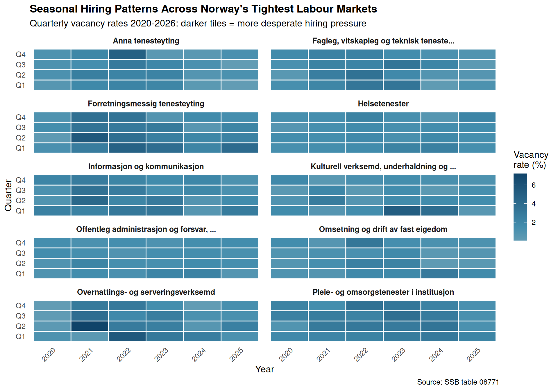
Healthcare and education show persistent dark tiles — chronically high vacancy rates across quarters and years. ICT and professional services show more volatility, with occasional cool-downs. Construction’s recent cooling is visible as lighter tiles in 2025-2026.
Healthcare crisis persists: Vacancy rates in health and social services remain above 3%, with thousands of unfilled positions creating service delivery strain across Norway’s municipalities.
Construction freeze deepens: Vacancy rates in building trades fell from 2.8% in early 2025 to 1.5% by Q1 2026, mirroring the housing market slowdown and suggesting further sector contraction ahead.
Professional services bifurcation: ICT and consulting maintain high vacancy rates (2.5-3%), but absolute counts have plateaued, indicating smaller but still talent-starved sectors.
Retail stabilization: After pandemic-era chaos, retail and wholesale vacancy rates have settled near 1.5% — low enough to suggest adequate labour supply but not so low as to signal hiring freezes.
Seasonal patterns eroding: Traditional Q1/Q4 hiring spikes are flattening in most sectors, possibly reflecting year-round recruitment as competition for workers intensifies.
The divergence between healthcare (chronic shortage) and construction (sudden cooling) suggests Norway’s labour market is fragmenting along structural lines. If vacancy rates in construction continue falling while healthcare stays elevated, it could signal a mismatch problem requiring active labour market policy — retraining programs, immigration policy shifts, or wage adjustments to redirect workers from contracting to expanding sectors. The next few quarters will show whether this is a temporary adjustment or a permanent realignment of Norwegian industry.