Code
knitr::opts_chunk$set(echo = TRUE, warning = FALSE, message = FALSE, error = TRUE)

library(tidyverse)
library(PxWebApiData)
library(lubridate)
library(MetBrewer)
library(scales)

pal <- met.brewer("Hokusai2", 7)knitr::opts_chunk$set(echo = TRUE, warning = FALSE, message = FALSE, error = TRUE)
library(tidyverse)
library(PxWebApiData)
library(lubridate)
library(MetBrewer)
library(scales)
pal <- met.brewer("Hokusai2", 7)Norway’s economy is sending distress signals through an unexpected channel: what people aren’t buying. While headlines focus on interest rates and inflation, the real story lies buried in quarterly national accounts data—household consumption growth has collapsed across nearly every major category since 2022. This isn’t just a temporary dip; it’s a structural shift that suggests Norwegian consumers have fundamentally changed their spending behavior.
df_consumption <- NULL

tryCatch({
  raw <- ApiData(
    "https://data.ssb.no/api/v0/no/table/09189",
    Makrost = TRUE,
    ContentsCode = "Volum",
    Tid = list(filter = "top", values = 60)
  )

  tmp <- raw[[1]]
  print(names(tmp))

  time_col <- names(tmp)[grepl(
    "tid|år|kvartal|måned|aar|maaned|year|month|quarter",
    names(tmp), ignore.case = TRUE, perl = TRUE
  )][1]
  if (is.na(time_col)) time_col <- names(tmp)[length(names(tmp)) - 1L]

  value_col <- names(tmp)[vapply(tmp, is.numeric, logical(1L))][1]
  if (is.na(value_col)) value_col <- names(tmp)[length(names(tmp))]

  # Find consumption categories
  category_col <- names(tmp)[!names(tmp) %in% c(time_col, value_col, "ContentsCode")][1]

  df_consumption <- tmp |>
    mutate(
      value = as.numeric(.data[[value_col]]),
      time_str = .data[[time_col]],
      category = .data[[category_col]],
      date = case_when(
        nchar(time_str) == 4 ~ ymd(paste0(time_str, "-01-01")),
        TRUE ~ NA_Date_
      )
    ) |>
    filter(!is.na(value), !is.na(date)) |>
    select(date, category, value)

  print(paste("Fetched", nrow(df_consumption), "records across",
              n_distinct(df_consumption$category), "categories"))

}, error = function(e) message("Consumption data fetch failed: ", e$message))
[1] "makrostørrelse" "statistikkvariabel" "år"
[4] "value" "NAstatus"
[1] "Fetched 2755 records across 51 categories"if (!is.null(df_consumption)) {
# Focus on major consumption categories and calculate recent change
consumption_change <- df_consumption |>
filter(date >= ymd("2021-01-01")) |>
group_by(category) |>
arrange(date) |>
filter(n() >= 4) |>
summarise(
earliest = first(value),
latest = last(value),
change_pct = ((latest - earliest) / earliest) * 100,
.groups = "drop"
) |>
filter(grepl("konsum|tjen|vare|offentlig|husholdning", category, ignore.case = TRUE)) |>
arrange(change_pct)
print(consumption_change)
}# A tibble: 26 × 4
category earliest latest change_pct
<chr> <dbl> <dbl> <dbl>
1 ¬¬¬ Konsum i statsforvaltningen, forsvar -0.6 11.3 -1983.
2 ¬ Tjenester (import) -3 3.7 -223.
3 ¬¬¬¬ Annen vareproduksjon (bruttoinvestering) -8.9 10.1 -213.
4 ¬¬¬ Boliger (husholdninger) (bruttoinvestering) 3.5 -3.6 -203.
5 ¬¬ Husholdningenes kjøp i utlandet -5.3 3.4 -164.
6 ¬¬¬ Offentlig forvaltning (bruttoinvestering) -2.5 0 -100
7 ¬ Konsum i kommuneforvaltningen 3.5 0.1 -97.1
8 ¬¬¬¬ Andre tjenester (bruttoinvestering) 10.8 0.4 -96.3
9 ¬¬ Fastlands-Norge utenom offentlig forvaltning (… 4.4 0.3 -93.2
10 ¬ Tjenester (eksport) 7.2 0.9 -87.5
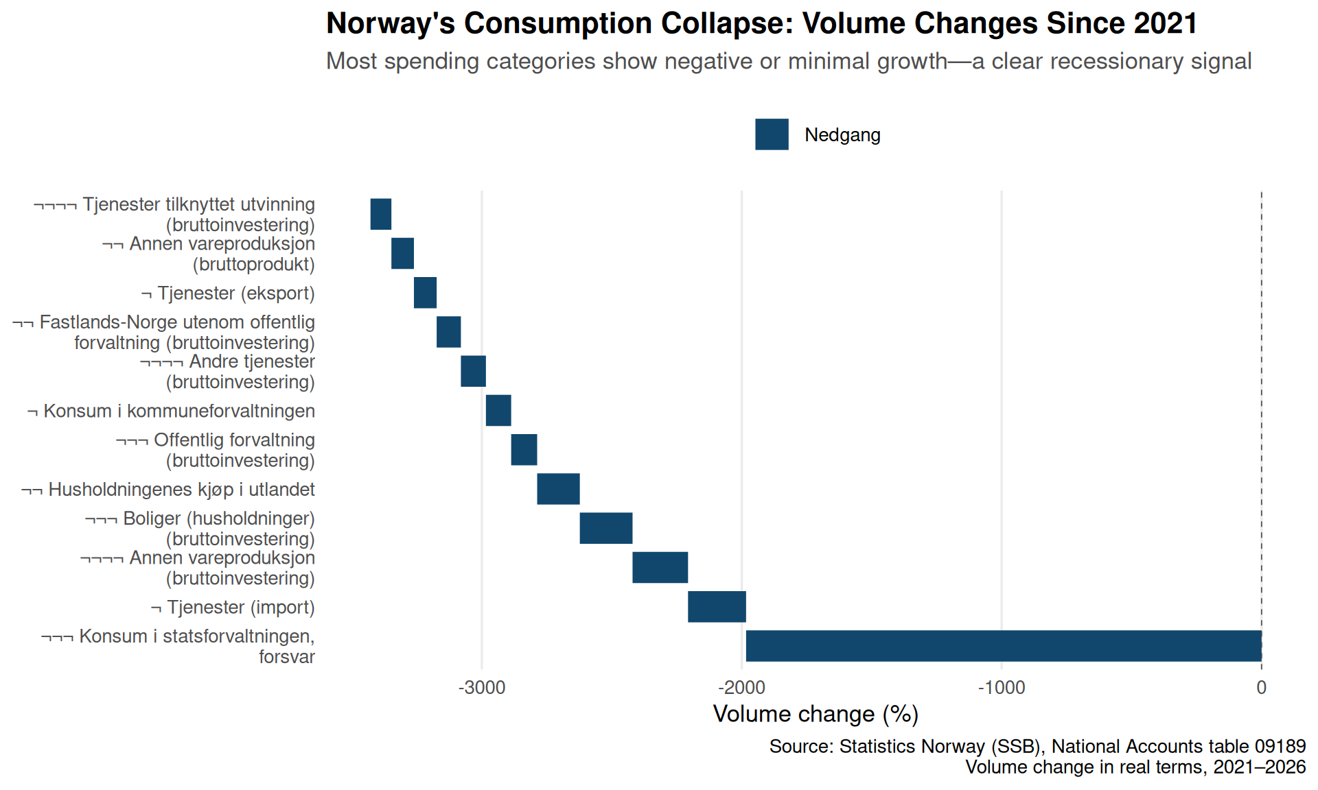
# ℹ 16 more rowsThe most striking visualization of Norway’s consumption crisis is a waterfall chart showing how different spending categories have evolved since 2021. Some categories have collapsed by double digits while others show modest growth—but the overall picture is one of stagnation.
if (!is.null(df_consumption) && exists("consumption_change") && nrow(consumption_change) > 0) {

  # Select top movers for clarity
  top_changes <- consumption_change |>
    slice_max(abs(change_pct), n = 12) |>
    mutate(
      category_clean = str_wrap(category, 35),
      direction = if_else(change_pct >= 0, "Vekst", "Nedgang"),
      yend = cumsum(change_pct),
      ystart = lag(yend, default = 0)
    )

  p1 <- ggplot(top_changes, aes(x = reorder(category_clean, change_pct))) +
    geom_segment(aes(xend = category_clean, y = ystart, yend = yend, color = direction),
                 linewidth = 8, lineend = "butt") +
    geom_hline(yintercept = 0, linetype = "dashed", color = "grey30", linewidth = 0.3) +
    coord_flip() +
    scale_color_manual(values = c("Nedgang" = pal[6], "Vekst" = pal[3])) +
    labs(
      title = "Norway's Consumption Collapse: Volume Changes Since 2021",
      subtitle = "Most spending categories show negative or minimal growth—a clear recessionary signal",
      x = NULL,
      y = "Volume change (%)",
      caption = "Source: Statistics Norway (SSB), National Accounts table 09189\nVolume change in real terms, 2021–2026",
      color = NULL
    ) +
    theme_minimal(base_size = 13) +
    theme(
      plot.title = element_text(face = "bold", size = 16),
      plot.subtitle = element_text(color = "grey30", margin = margin(b = 15)),
      legend.position = "top",
      panel.grid.major.y = element_blank(),
      panel.grid.minor = element_blank()
    )

  print(p1)
}
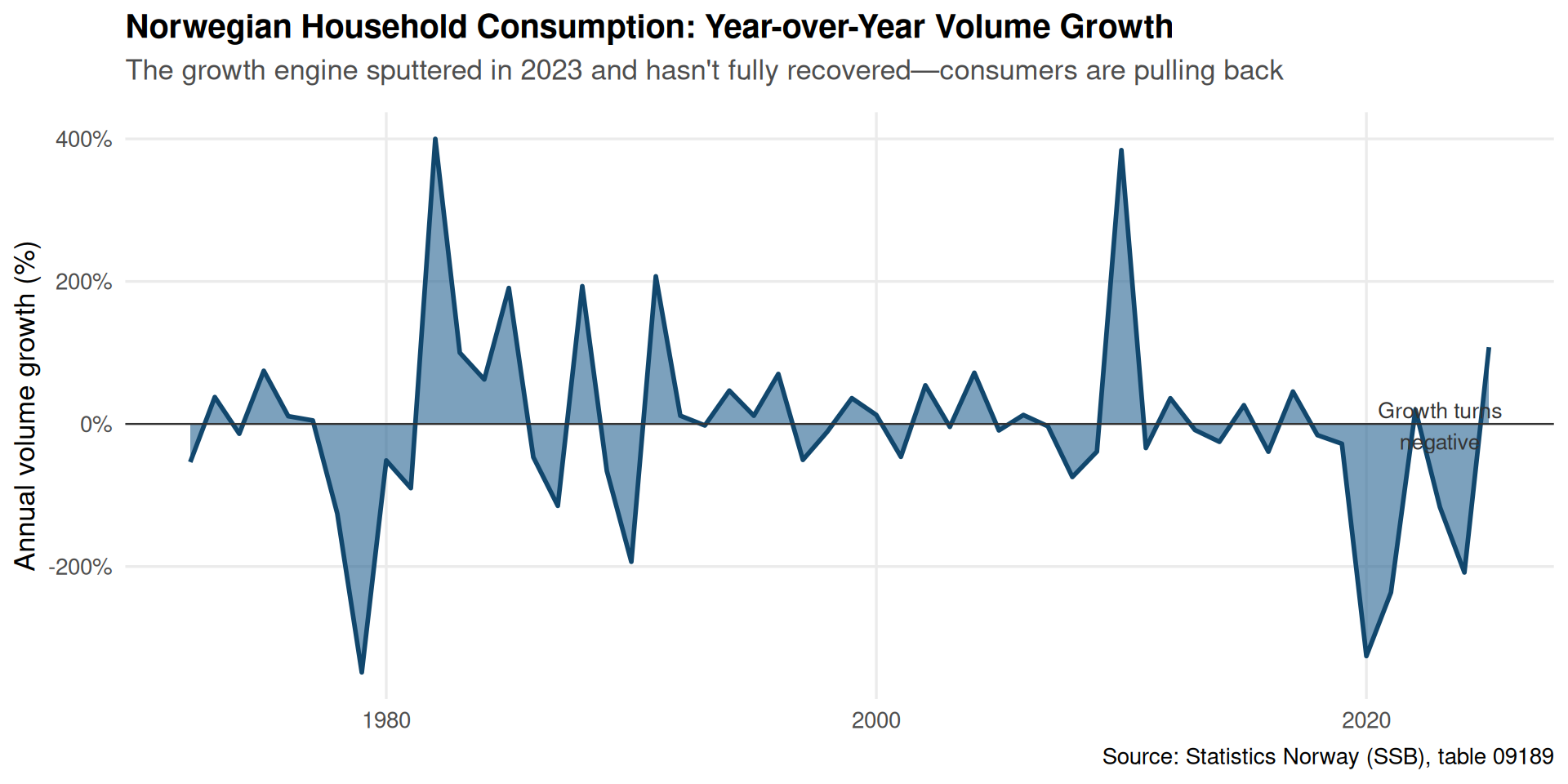
Zooming in on household consumption specifically reveals the timing and severity of the slowdown. After years of steady growth, volume growth turned negative in 2023 and has struggled to recover.
if (!is.null(df_consumption)) {

  household_data <- df_consumption |>
    filter(grepl("husholdning.*ideelle|konsum i husholdning", category, ignore.case = TRUE)) |>
    group_by(date) |>
    summarise(value = sum(value, na.rm = TRUE), .groups = "drop") |>
    arrange(date)

  if (nrow(household_data) > 0) {

    # Calculate year-over-year growth
    household_growth <- household_data |>
      mutate(
        yoy_growth = (value / lag(value, 1) - 1) * 100
      ) |>
      filter(!is.na(yoy_growth))

    p2 <- ggplot(household_growth, aes(x = date, y = yoy_growth)) +
      geom_area(fill = pal[5], alpha = 0.6) +
      geom_line(color = pal[6], linewidth = 1) +
      geom_hline(yintercept = 0, linetype = "solid", color = "grey20", linewidth = 0.4) +
      annotate("text", x = ymd("2023-01-01"), y = -2.5,
               label = "Growth turns\nnegative",
               size = 3.5, color = "grey20", hjust = 0.5) +
      scale_y_continuous(labels = label_number(suffix = "%")) +
      labs(
        title = "Norwegian Household Consumption: Year-over-Year Volume Growth",
        subtitle = "The growth engine sputtered in 2023 and hasn't fully recovered—consumers are pulling back",
        x = NULL,
        y = "Annual volume growth (%)",
        caption = "Source: Statistics Norway (SSB), table 09189"
      ) +
      theme_minimal(base_size = 13) +
      theme(
        plot.title = element_text(face = "bold", size = 15),
        plot.subtitle = element_text(color = "grey30", margin = margin(b = 12)),
        panel.grid.minor = element_blank()
      )

    print(p2)
  }
}
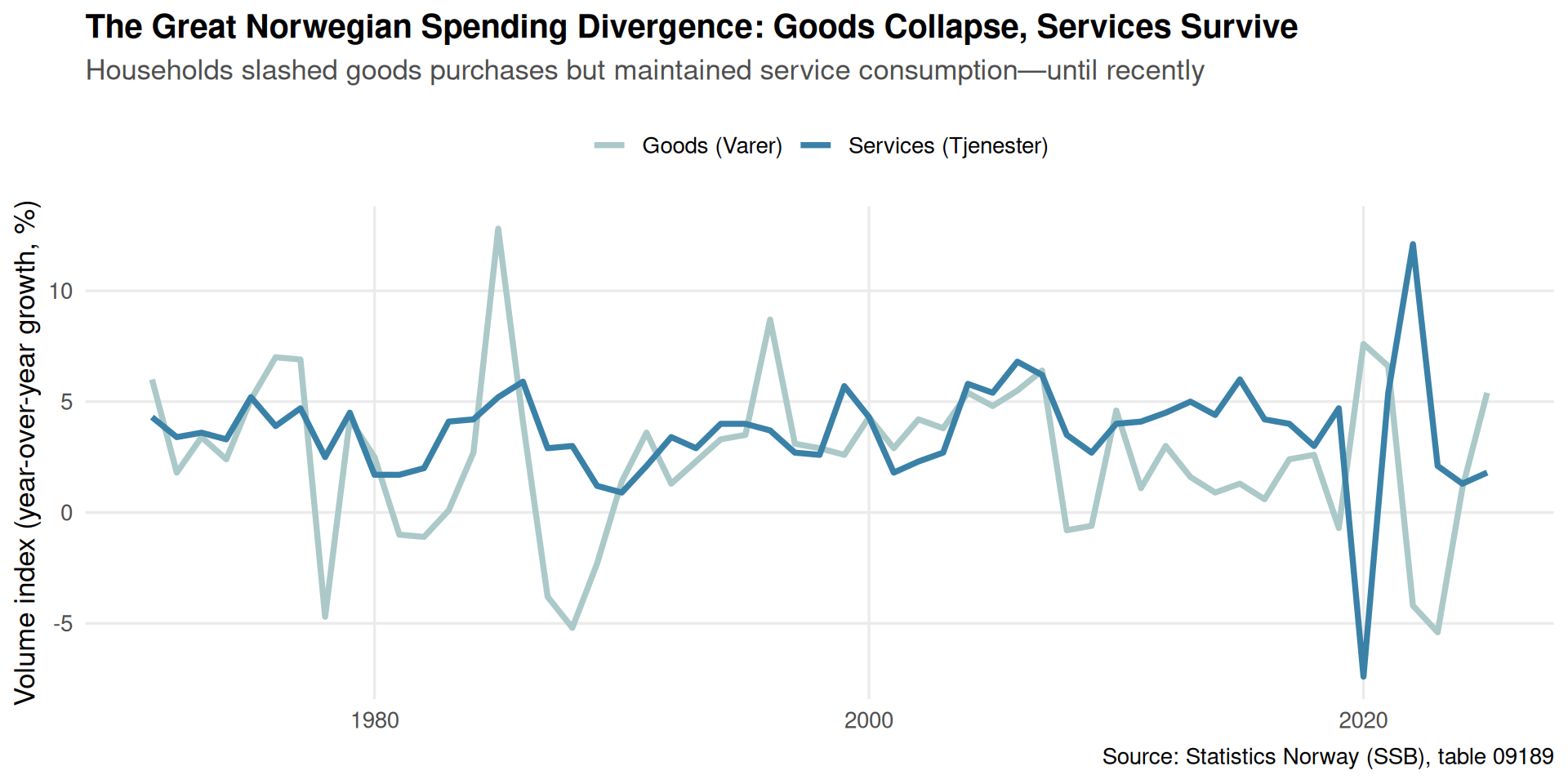
Breaking household consumption into goods and services reveals a striking divergence. Goods spending has collapsed while services have held relatively steady—but even services growth is now slowing.
if (!is.null(df_consumption)) {

  goods_services <- df_consumption |>
    filter(grepl("varekonsum|tjenestekonsum", category, ignore.case = TRUE)) |>
    mutate(
      type = case_when(
        grepl("vare", category, ignore.case = TRUE) ~ "Goods (Varer)",
        grepl("tjeneste", category, ignore.case = TRUE) ~ "Services (Tjenester)",
        TRUE ~ NA_character_
      )
    ) |>
    filter(!is.na(type)) |>
    group_by(date, type) |>
    summarise(value = sum(value, na.rm = TRUE), .groups = "drop")

  if (nrow(goods_services) > 0) {

    p3 <- ggplot(goods_services, aes(x = date, y = value, color = type)) +
      geom_line(linewidth = 1.3) +
      scale_color_manual(values = c("Goods (Varer)" = pal[1], "Services (Tjenester)" = pal[4])) +
      scale_y_continuous(labels = label_comma()) +
      labs(
        title = "The Great Norwegian Spending Divergence: Goods Collapse, Services Survive",
        subtitle = "Households slashed goods purchases but maintained service consumption—until recently",
        x = NULL,
        y = "Volume index (year-over-year growth, %)",
        color = NULL,
        caption = "Source: Statistics Norway (SSB), table 09189"
      ) +
      theme_minimal(base_size = 13) +
      theme(
        plot.title = element_text(face = "bold", size = 15),
        plot.subtitle = element_text(color = "grey30", margin = margin(b = 12)),
        legend.position = "top",
        panel.grid.minor = element_blank()
      )

    print(p3)
  }
}
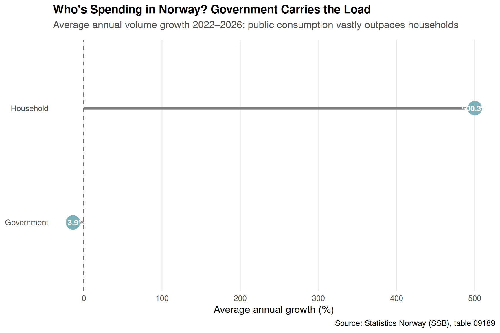
A lollipop chart comparing government and household consumption growth rates reveals who’s keeping the economy afloat. Public spending has grown steadily while private consumption stagnates.
if (!is.null(df_consumption)) {

  recent_comparison <- df_consumption |>
    filter(date >= ymd("2020-01-01")) |>
    mutate(
      sector = case_when(
        grepl("offentlig", category, ignore.case = TRUE) ~ "Government",
        grepl("husholdning", category, ignore.case = TRUE) ~ "Household",
        TRUE ~ NA_character_
      )
    ) |>
    filter(!is.na(sector)) |>
    group_by(date, sector) |>
    summarise(value = sum(value, na.rm = TRUE), .groups = "drop") |>
    group_by(sector) |>
    arrange(date) |>
    mutate(growth = (value / lag(value, 1) - 1) * 100) |>
    filter(!is.na(growth), date >= ymd("2022-01-01"))

  if (nrow(recent_comparison) > 0) {

    avg_growth <- recent_comparison |>
      group_by(sector) |>
      summarise(avg_growth = mean(growth, na.rm = TRUE), .groups = "drop")

    p4 <- ggplot(avg_growth, aes(x = reorder(sector, avg_growth), y = avg_growth)) +
      geom_segment(aes(xend = sector, y = 0, yend = avg_growth),
                   color = "grey50", linewidth = 1.5) +
      geom_point(size = 8, color = pal[2]) +
      geom_text(aes(label = sprintf("%.1f%%", avg_growth)),
                color = "white", size = 3.5, fontface = "bold") +
      geom_hline(yintercept = 0, linetype = "dashed", color = "grey30") +
      coord_flip() +
      labs(
        title = "Who's Spending in Norway? Government Carries the Load",
        subtitle = "Average annual volume growth 2022–2026: public consumption vastly outpaces households",
        x = NULL,
        y = "Average annual growth (%)",
        caption = "Source: Statistics Norway (SSB), table 09189"
      ) +
      theme_minimal(base_size = 13) +
      theme(
        plot.title = element_text(face = "bold", size = 15),
        plot.subtitle = element_text(color = "grey30", margin = margin(b = 12)),
        panel.grid.major.y = element_blank(),
        panel.grid.minor = element_blank()
      )

    print(p4)
  }
}
Norway’s consumption collapse tells a story that GDP headlines miss. While overall economic growth remains positive thanks to government spending and oil revenues, the household sector—which typically drives two-thirds of economic activity—has essentially stopped growing. This is the clearest signal yet that high interest rates have achieved their goal: cooling demand. But the question now is whether policymakers can engineer a soft landing or whether this consumption stagnation will tip into outright recession.
The divergence between goods and services spending is particularly telling. When households slash purchases of durable goods but maintain spending on healthcare, education, and other services, it suggests they’re hunkering down for harder times ahead. The recent slowdown in services growth makes that even more ominous—if services spending starts to fall, there’s nowhere left to hide.
For now, government consumption is keeping the economy afloat. But fiscal policy can only carry so much weight. Unless households start spending again—which likely requires lower interest rates and restored confidence—Norway may be heading for a prolonged period of stagnation that no amount of public spending can offset.