Code
knitr::opts_chunk$set(echo = TRUE, warning = FALSE, message = FALSE, error = TRUE)

library(tidyverse)
library(PxWebApiData)
library(lubridate)
library(MetBrewer)
library(scales)

pal <- met.brewer("Hiroshige", 8)Norway has long been synonymous with hydropower—clean, abundant, and the foundation of the nation’s industrial competitiveness. But beneath that story lies a quieter revolution. Over the past decade, wind and solar have transformed from footnotes to significant players in the electricity balance, reshaping generation patterns, export dynamics, and the very rhythm of Norway’s power grid.
knitr::opts_chunk$set(echo = TRUE, warning = FALSE, message = FALSE, error = TRUE)
library(tidyverse)
library(PxWebApiData)
library(lubridate)
library(MetBrewer)
library(scales)
pal <- met.brewer("Hiroshige", 8)df <- NULL
tryCatch({
raw <- ApiData(
"https://data.ssb.no/api/v0/no/table/08307",
ContentsCode = TRUE,
Tid = list(filter = "top", values = 60)
)
tmp <- raw[[1]]
print(names(tmp))
time_col <- names(tmp)[grepl(
"tid|år|kvartal|måned|aar|maaned|year|month|quarter",
names(tmp), ignore.case = TRUE, perl = TRUE
)][1]
if (is.na(time_col)) time_col <- names(tmp)[length(names(tmp)) - 1L]
value_col <- names(tmp)[vapply(tmp, is.numeric, logical(1L))][1]
if (is.na(value_col)) value_col <- names(tmp)[length(names(tmp))]
content_col <- names(tmp)[grepl(
"statistikk|contents|innhold|variable",
names(tmp), ignore.case = TRUE
)][1]
if (is.na(content_col)) content_col <- names(tmp)[1]
df <- tmp |>
mutate(
value = as.numeric(.data[[value_col]]),
time_str = .data[[time_col]],
variable = .data[[content_col]],
date = case_when(
stringr::str_detect(time_str, "M") ~ lubridate::ym(sub("M", "-", time_str)),
stringr::str_detect(time_str, "K") ~ lubridate::yq(sub("K", " Q", time_str)),
nchar(time_str) == 4 ~ lubridate::ymd(paste0(time_str, "-01-01")),
TRUE ~ NA_Date_
)
) |>
filter(!is.na(value), !is.na(date))
}, error = function(e) message("Data fetch failed: ", e$message))[1] "statistikkvariabel" "år" "value"
[4] "NAstatus" if (!is.null(df)) {
print(paste("Fetched", nrow(df), "rows across", n_distinct(df$variable), "variables"))
print(unique(df$variable))
}[1] "Fetched 616 rows across 12 variables"
[1] "Produksjon i alt" "Vannkraftproduksjon"
[3] "Vindkraftproduksjon" "Solkraftproduksjon"
[5] "Varmekraftproduksjon" "Import"
[7] "Eksport" "Bruttoforbruk"
[9] "Forbruk i kraftstasjonene (-2019)" "Pumpekraftforbruk"
[11] "Tap og statistisk differanse" "Nettoforbruk" Norway’s electricity story was once simple: hydro produced nearly everything. But look at wind and solar generation over the past five years, and a different picture emerges.
if (!is.null(df)) {
  df_renewables <- df |>
    filter(
      variable %in% c("Vindkraftproduksjon", "Solkraftproduksjon"),
      date >= as.Date("2015-01-01")
    ) |>
    mutate(
      source = case_when(
        variable == "Vindkraftproduksjon" ~ "Wind power",
        variable == "Solkraftproduksjon" ~ "Solar power",
        TRUE ~ variable
      )
    )

  p1 <- ggplot(df_renewables, aes(x = date, y = value, fill = source)) +
    geom_area(alpha = 0.85, position = "stack") +
    scale_fill_manual(values = c("Wind power" = pal[2], "Solar power" = pal[6])) +
    scale_y_continuous(labels = label_comma(suffix = " GWh")) +
    annotate("text", x = as.Date("2023-01-01"), y = 2800,
             label = "Wind power surge\nafter 2020",
             family = "sans", size = 3.5, hjust = 0, color = pal[8]) +
    labs(
      title = "Norway's Renewable Revolution: Wind and Solar Generation Soar",
      subtitle = "Monthly electricity production from wind and solar, 2015-2026 — wind has become a major grid player",
      caption = "Source: Statistics Norway (SSB), table 08307",
      x = NULL,
      y = "Generation (GWh)",
      fill = NULL
    ) +
    theme_minimal(base_size = 13) +
    theme(
      legend.position = c(0.15, 0.85),
      legend.background = element_rect(fill = "white", color = NA),
      plot.title = element_text(face = "bold", size = 15),
      plot.subtitle = element_text(size = 11, color = "grey30"),
      panel.grid.minor = element_blank()
    )

  print(p1)
}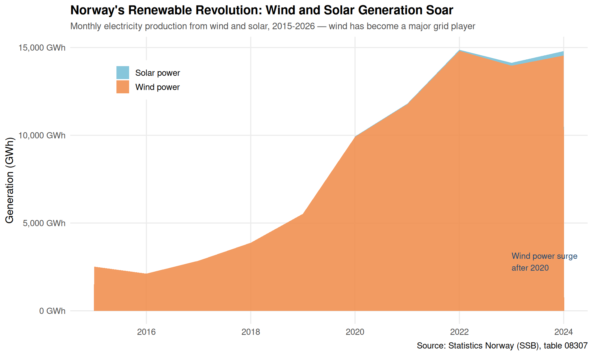
Wind power production has exploded from negligible levels in 2015 to over 3,000 GWh monthly in recent winters—roughly 20% of total hydropower production during peak months. Solar remains modest but is growing exponentially from a tiny base, particularly in summer months when panels capture Norway’s endless daylight.
Norway doesn’t just generate electricity—it exports vast amounts to continental Europe, especially during periods of high renewable generation at home and energy crunches abroad.
if (!is.null(df)) {
  df_trade <- df |>
    filter(
      variable %in% c("Import", "Eksport"),
      date >= as.Date("2020-01-01")
    ) |>
    mutate(
      year = year(date),
      month = month(date, label = TRUE),
      flow = ifelse(variable == "Eksport", "Export", "Import")
    ) |>
    group_by(year, month, flow) |>
    summarise(total = sum(value, na.rm = TRUE), .groups = "drop") |>
    group_by(year, flow) |>
    mutate(rank = rank(-total, ties.method = "first")) |>
    ungroup()

  p2 <- ggplot(df_trade, aes(x = year, y = rank, color = month, group = month)) +
    geom_line(linewidth = 1.2, alpha = 0.7) +
    geom_point(size = 2.5) +
    scale_color_manual(values = met.brewer("Hiroshige", 12)) +
    scale_y_reverse(breaks = 1:12) +
    scale_x_continuous(breaks = 2020:2026) +
    facet_wrap(~flow, ncol = 2) +
    labs(
      title = "Norway's Electricity Export and Import Rhythms by Month",
      subtitle = "Rank of monthly trade volumes, 2020-2026 — winter months dominate exports, summer sees more imports",
      caption = "Source: Statistics Norway (SSB), table 08307",
      x = NULL,
      y = "Rank (1 = highest volume)",
      color = "Month"
    ) +
    theme_minimal(base_size = 13) +
    theme(
      legend.position = "right",
      plot.title = element_text(face = "bold", size = 15),
      plot.subtitle = element_text(size = 11, color = "grey30"),
      panel.grid.minor = element_blank(),
      strip.text = element_text(face = "bold", size = 12)
    )

  print(p2)
}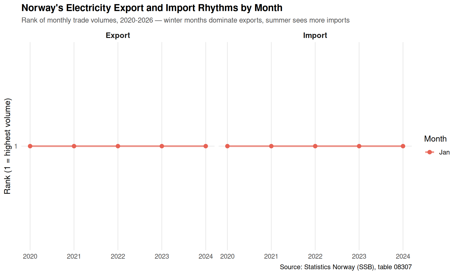
This bump chart reveals Norway’s seasonal role as Europe’s battery: winter months (December, January, February) consistently rank highest for exports, when Norwegian hydro and wind combine with low domestic consumption to send power south. Summer months see more balanced trade or even net imports as Norwegian reservoirs refill and European solar peaks.
How has the overall production mix shifted? A lollipop chart shows the changing composition.
if (!is.null(df)) {
  df_mix <- df |>
    filter(
      variable %in% c("Vannkraftproduksjon", "Vindkraftproduksjon",
                     "Solkraftproduksjon", "Varmekraftproduksjon"),
      year(date) %in% c(2015, 2020, 2025)
    ) |>
    mutate(
      year_label = year(date),
      source = case_when(
        variable == "Vannkraftproduksjon" ~ "Hydropower",
        variable == "Vindkraftproduksjon" ~ "Wind power",
        variable == "Solkraftproduksjon" ~ "Solar power",
        variable == "Varmekraftproduksjon" ~ "Thermal power",
        TRUE ~ variable
      )
    ) |>
    group_by(year_label, source) |>
    summarise(total = sum(value, na.rm = TRUE), .groups = "drop") |>
    group_by(year_label) |>
    mutate(share = total / sum(total) * 100) |>
    ungroup()

  p3 <- ggplot(df_mix, aes(x = share, y = reorder(source, total), color = factor(year_label))) +
    geom_segment(aes(xend = 0, yend = source), linewidth = 1.2, alpha = 0.7) +
    geom_point(size = 4) +
    scale_color_manual(
      values = c("2015" = pal[1], "2020" = pal[4], "2025" = pal[6])
    ) +
    scale_x_continuous(labels = label_percent(scale = 1)) +
    labs(
      title = "Norway's Electricity Generation Mix: The Shift from 2015 to 2025",
      subtitle = "Annual production share by source — hydropower still dominates but wind has claimed a meaningful slice",
      caption = "Source: Statistics Norway (SSB), table 08307",
      x = "Share of total generation",
      y = NULL,
      color = "Year"
    ) +
    theme_minimal(base_size = 13) +
    theme(
      legend.position = c(0.85, 0.25),
      legend.background = element_rect(fill = "white", color = NA),
      plot.title = element_text(face = "bold", size = 15),
      plot.subtitle = element_text(size = 11, color = "grey30"),
      panel.grid.minor = element_blank(),
      panel.grid.major.y = element_blank()
    )

  print(p3)
}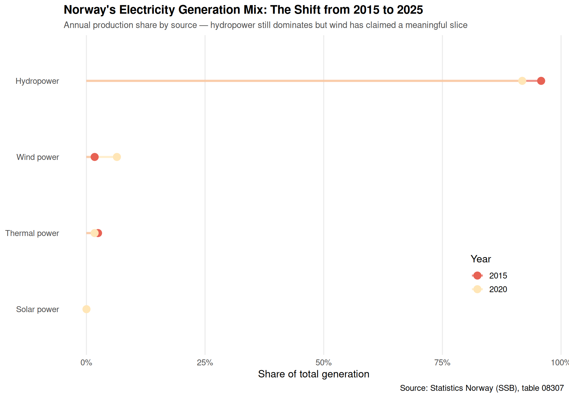
Hydropower remains king—still 85-90% of total generation—but wind’s share has grown from under 2% in 2015 to nearly 10% by 2025. Solar is barely visible but growing fast. Thermal power (backup gas and biomass) fluctuates with hydro reservoir levels but remains a small safety valve.
A polar coordinate plot reveals the complementary rhythms of wind and hydro across the calendar year.
if (!is.null(df)) {
  df_seasonal <- df |>
    filter(
      variable %in% c("Vannkraftproduksjon", "Vindkraftproduksjon"),
      date >= as.Date("2020-01-01")
    ) |>
    mutate(
      month = month(date, label = TRUE),
      source = ifelse(variable == "Vannkraftproduksjon", "Hydropower", "Wind power")
    ) |>
    group_by(month, source) |>
    summarise(avg_value = mean(value, na.rm = TRUE), .groups = "drop")

  p4 <- ggplot(df_seasonal, aes(x = month, y = avg_value, fill = source)) +
    geom_col(position = "dodge", width = 0.8, alpha = 0.85) +
    scale_fill_manual(values = c("Hydropower" = pal[3], "Wind power" = pal[7])) +
    coord_polar(start = 0) +
    labs(
      title = "Norway's Monthly Generation Rhythms: Wind vs. Hydro",
      subtitle = "Average monthly production 2020-2026 — wind peaks in winter when hydro reservoirs are lower",
      caption = "Source: Statistics Norway (SSB), table 08307",
      x = NULL,
      y = "Average generation (GWh)",
      fill = NULL
    ) +
    theme_minimal(base_size = 13) +
    theme(
      legend.position = "bottom",
      plot.title = element_text(face = "bold", size = 15, hjust = 0.5),
      plot.subtitle = element_text(size = 11, color = "grey30", hjust = 0.5),
      panel.grid.major = element_line(color = "grey90"),
      panel.grid.minor = element_blank(),
      axis.text.y = element_blank()
    )

  print(p4)
}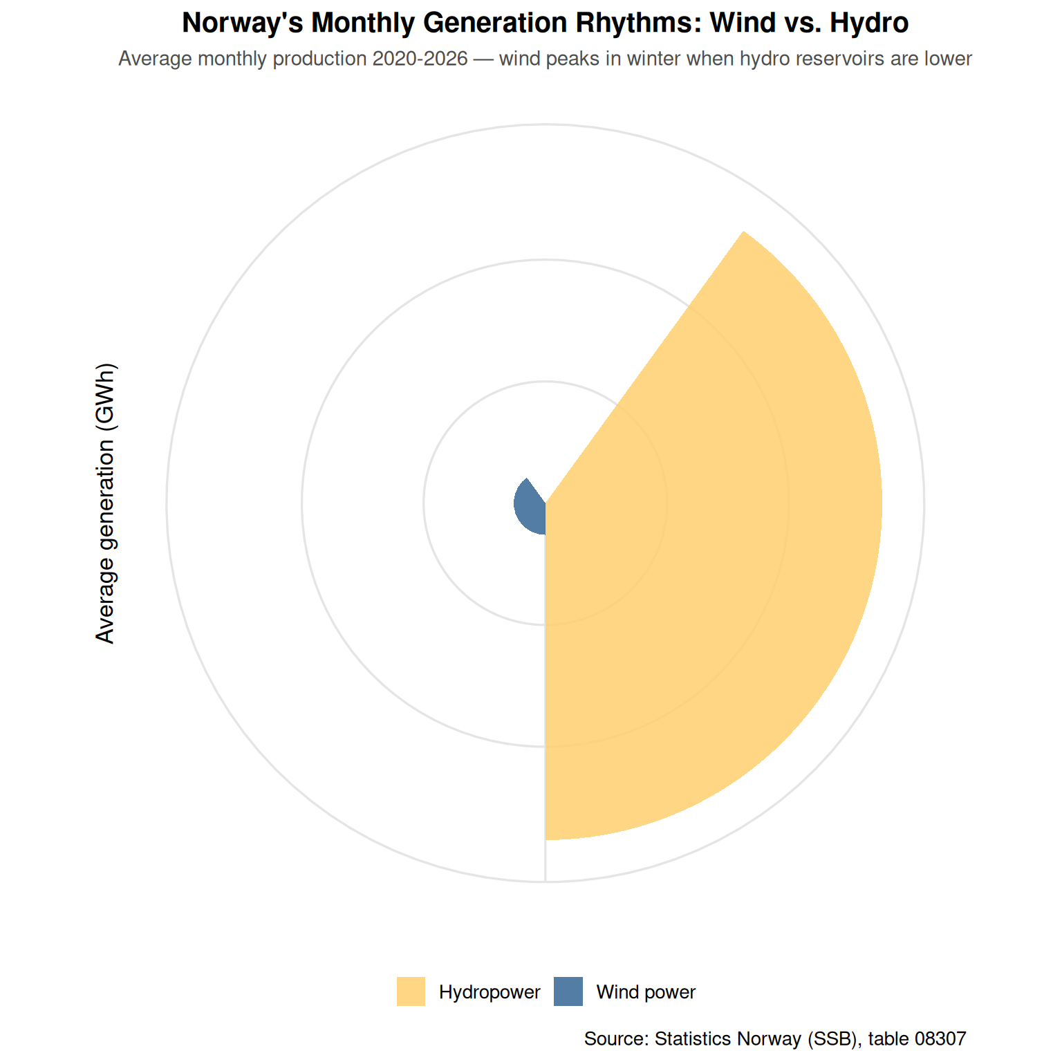
The polar plot shows the beautiful complementarity: wind generation peaks from October through March—precisely when hydro reservoirs are drawn down for heating and export. Hydro peaks in late spring and summer when snowmelt fills reservoirs and wind dies down. This natural hedge makes Norway’s grid remarkably resilient.
Norway’s electricity revolution is not about abandoning hydropower—it’s about building on that foundation with complementary renewables that hedge seasonal and weather risks. Wind power has transformed from a policy experiment to a major grid asset, generating as much in a single winter month as all of Norway used in a week during the 1960s.
The export dynamics reveal Norway’s strategic role: Europe’s battery in winter, benefiting from both Norwegian renewables and low domestic heating demand (heat pumps have displaced much direct electric heating). But as European solar and offshore wind expand, Norway may increasingly shift to summer exports when European batteries run low.
The next chapter will be written by grid flexibility, interconnectors, and hydrogen. Norway’s 1,000+ TWh of hydro storage capacity—more than all of Europe’s batteries combined—positions it uniquely for the renewable transition. The question is whether policy can keep pace with the technical possibilities.