Code
knitr::opts_chunk$set(echo = TRUE, warning = FALSE, message = FALSE, error = TRUE)
library(tidyverse)
library(PxWebApiData)
library(lubridate)
library(MetBrewer)
library(scales)
pal <- met.brewer("Hiroshige", 8)March 26, 2026
What Norwegians choose to spend their money on tells a more intimate economic story than any GDP figure. Over the past three decades, household consumption patterns have undergone a quiet revolution — from what we eat and drive to how we heat our homes and entertain ourselves. This transformation reveals structural shifts in the Norwegian economy that official growth statistics alone cannot capture.
We begin with the comprehensive national accounts data on household final consumption expenditure, tracking major spending categories since the early 1990s.
df_cons <- NULL
tryCatch({
raw <- ApiData(
"https://data.ssb.no/api/v0/no/table/11174",
Region = "0",
Kjopegrupper = TRUE,
PetroleumProd = "00",
ContentsCode = TRUE,
Tid = list(filter = "top", values = 120)
)
tmp <- raw[[1]]
print(names(tmp))
time_col <- names(tmp)[grepl(
"tid|år|kvartal|måned|aar|maaned|year|month|quarter",
names(tmp), ignore.case = TRUE, perl = TRUE
)][1]
if (is.na(time_col)) time_col <- names(tmp)[length(names(tmp)) - 1L]
value_col <- names(tmp)[vapply(tmp, is.numeric, logical(1L))][1]
if (is.na(value_col)) value_col <- names(tmp)[length(names(tmp))]
df_cons <- tmp |>
mutate(
value = as.numeric(.data[[value_col]]),
time_str = .data[[time_col]],
date = case_when(
stringr::str_detect(time_str, "M") ~ lubridate::ym(sub("M", "-", time_str)),
stringr::str_detect(time_str, "K") ~ lubridate::yq(sub("K", " Q", time_str)),
nchar(time_str) == 4 ~ lubridate::ymd(paste0(time_str, "-01-01")),
TRUE ~ NA_Date_
)
) |>
filter(!is.na(value), !is.na(date))
}, error = function(e) message("Consumption data fetch failed: ", e$message))[1] "region" "kjøpegruppe" "petroleumsprodukt"
[4] "statistikkvariabel" "måned" "value"
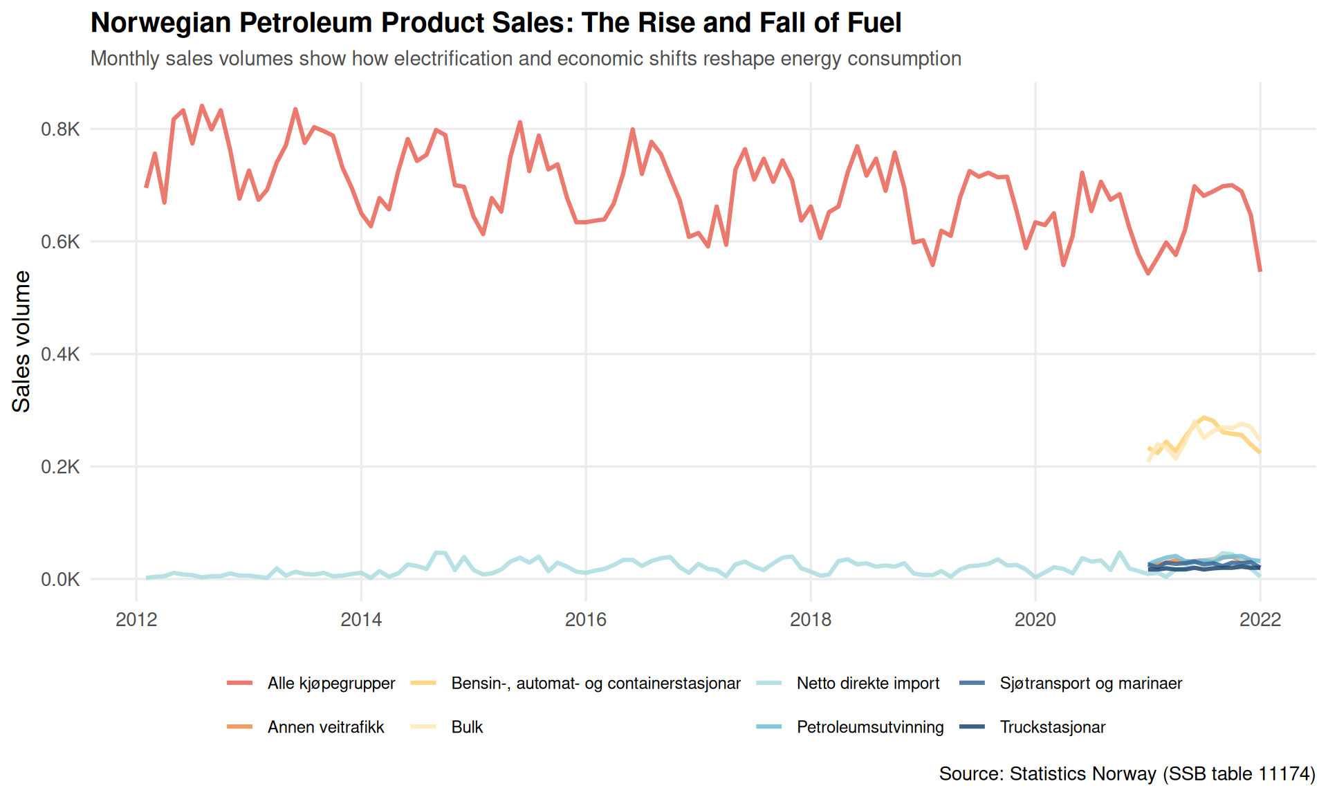
[7] "NAstatus"
The petroleum product sales data captures one critical piece of Norway’s consumption story — fuel patterns that reflect everything from electric vehicle adoption to economic cycles.
if (!is.null(df_cons)) {
# Detect category column
cat_col <- names(df_cons)[grepl("kjope|gruppe|category", names(df_cons), ignore.case = TRUE)][1]
if (!is.na(cat_col)) {
# Focus on major fuel categories
df_fuel <- df_cons |>
filter(!is.na(.data[[cat_col]]),
year(date) >= 2010)
# Get top categories by recent volume
top_cats <- df_fuel |>
filter(date >= max(date) - years(1)) |>
group_by(across(all_of(cat_col))) |>
summarize(avg_val = mean(value, na.rm = TRUE), .groups = "drop") |>
arrange(desc(avg_val)) |>
head(8) |>
pull(cat_col)
df_plot <- df_fuel |>
filter(.data[[cat_col]] %in% top_cats)
p1 <- ggplot(df_plot, aes(x = date, y = value, color = .data[[cat_col]])) +
geom_line(linewidth = 1.1, alpha = 0.85) +
scale_color_manual(values = pal, name = NULL) +
scale_y_continuous(labels = label_number(scale = 1e-3, suffix = "K")) +
labs(
title = "Norwegian Petroleum Product Sales: The Rise and Fall of Fuel",
subtitle = "Monthly sales volumes show how electrification and economic shifts reshape energy consumption",
x = NULL,
y = "Sales volume",
caption = "Source: Statistics Norway (SSB table 11174)"
) +
theme_minimal(base_size = 13) +
theme(
legend.position = "bottom",
legend.text = element_text(size = 9),
plot.title = element_text(face = "bold", size = 15),
plot.subtitle = element_text(color = "gray30", size = 11),
panel.grid.minor = element_blank()
) +
guides(color = guide_legend(nrow = 2))
print(p1)
}
}
Moving beyond petroleum, we examine the broader national accounts data to understand how total household consumption has evolved relative to other economic aggregates.
df_na <- NULL
tryCatch({
raw <- ApiData(
"https://data.ssb.no/api/v0/no/table/12880",
ContentsCode = c("KonsumHushold", "KonsumOffentl", "BtoInvFastReal",
"BNP", "BNPFastlands"),
Tid = list(filter = "top", values = 35)
)
tmp <- raw[[1]]
print(names(tmp))
time_col <- names(tmp)[grepl(
"tid|år|kvartal|måned|aar|maaned|year|month|quarter",
names(tmp), ignore.case = TRUE, perl = TRUE
)][1]
if (is.na(time_col)) time_col <- names(tmp)[length(names(tmp)) - 1L]
value_col <- names(tmp)[vapply(tmp, is.numeric, logical(1L))][1]
if (is.na(value_col)) value_col <- names(tmp)[length(names(tmp))]
cat_col <- names(tmp)[grepl("contents|innhold|statistikk", names(tmp), ignore.case = TRUE)][1]
df_na <- tmp |>
mutate(
value = as.numeric(.data[[value_col]]),
time_str = .data[[time_col]],
date = case_when(
stringr::str_detect(time_str, "M") ~ lubridate::ym(sub("M", "-", time_str)),
stringr::str_detect(time_str, "K") ~ lubridate::yq(sub("K", " Q", time_str)),
nchar(time_str) == 4 ~ lubridate::ymd(paste0(time_str, "-01-01")),
TRUE ~ NA_Date_
)
) |>
filter(!is.na(value), !is.na(date))
}, error = function(e) message("National accounts fetch failed: ", e$message))if (!is.null(df_na)) {
cat_col <- names(df_na)[grepl("contents|innhold|statistikk", names(df_na), ignore.case = TRUE)][1]
if (!is.na(cat_col)) {
# Calculate shares relative to GDP
df_shares <- df_na |>
filter(!is.na(.data[[cat_col]])) |>
group_by(date) |>
mutate(
gdp = value[grepl("BNP", .data[[cat_col]], ignore.case = TRUE) &
!grepl("Fastland", .data[[cat_col]], ignore.case = TRUE)][1],
share = (value / gdp) * 100
) |>
ungroup() |>
filter(!grepl("BNP", .data[[cat_col]], ignore.case = TRUE))
p2 <- ggplot(df_shares, aes(x = date, y = share, fill = .data[[cat_col]])) +
geom_area(alpha = 0.7, color = "white", linewidth = 0.3) +
scale_fill_manual(values = pal[c(1, 3, 5)], name = NULL) +
scale_y_continuous(labels = label_percent(scale = 1)) +
labs(
title = "How Norway Spends Its GDP: The Composition Shift",
subtitle = "Household consumption, government spending, and investment as shares of total GDP",
x = NULL,
y = "Share of GDP (%)",
caption = "Source: Statistics Norway (SSB table 12880)"
) +
theme_minimal(base_size = 13) +
theme(
legend.position = "bottom",
plot.title = element_text(face = "bold", size = 15),
plot.subtitle = element_text(color = "gray30", size = 11),
panel.grid.minor = element_blank()
)
print(p2)
}
}Consumer prices tell the other half of the consumption story. The new Consumer Price Index series lets us see exactly which spending categories have faced the steepest inflation.
df_cpi <- NULL
tryCatch({
raw <- ApiData(
"https://data.ssb.no/api/v0/no/table/14700",
VareTjenesteGrp = c("00", "01", "02", "03", "04", "05", "06", "07", "08", "09", "10", "11", "12"),
ContentsCode = "Tolvmanedersendring",
Tid = list(filter = "top", values = 60)
)
tmp <- raw[[1]]
print(names(tmp))
time_col <- names(tmp)[grepl(
"tid|år|kvartal|måned|aar|maaned|year|month|quarter",
names(tmp), ignore.case = TRUE, perl = TRUE
)][1]
if (is.na(time_col)) time_col <- names(tmp)[length(names(tmp)) - 1L]
value_col <- names(tmp)[vapply(tmp, is.numeric, logical(1L))][1]
if (is.na(value_col)) value_col <- names(tmp)[length(names(tmp))]
df_cpi <- tmp |>
mutate(
value = as.numeric(.data[[value_col]]),
time_str = .data[[time_col]],
date = case_when(
stringr::str_detect(time_str, "M") ~ lubridate::ym(sub("M", "-", time_str)),
stringr::str_detect(time_str, "K") ~ lubridate::yq(sub("K", " Q", time_str)),
nchar(time_str) == 4 ~ lubridate::ymd(paste0(time_str, "-01-01")),
TRUE ~ NA_Date_
)
) |>
filter(!is.na(value), !is.na(date))
}, error = function(e) message("CPI data fetch failed: ", e$message))[1] "vare- og tjenestegruppe" "statistikkvariabel"
[3] "måned" "value"
if (!is.null(df_cpi)) {
cat_col <- names(df_cpi)[grepl("vare|tjeneste|gruppe|category", names(df_cpi), ignore.case = TRUE)][1]
if (!is.na(cat_col)) {
# Exclude total, focus on main categories
df_plot_cpi <- df_cpi |>
filter(!is.na(.data[[cat_col]]),
!grepl("^00$|I alt", .data[[cat_col]], ignore.case = TRUE))
# Get recent inflation rates for ordering
recent_inflation <- df_plot_cpi |>
filter(date >= max(date) - months(6)) |>
group_by(across(all_of(cat_col))) |>
summarize(avg_inflation = mean(value, na.rm = TRUE), .groups = "drop") |>
arrange(desc(avg_inflation))
df_plot_cpi <- df_plot_cpi |>
mutate(category_ordered = factor(.data[[cat_col]],
levels = recent_inflation[[cat_col]]))
p3 <- ggplot(df_plot_cpi, aes(x = date, y = value, color = category_ordered)) +
geom_line(linewidth = 0.9, alpha = 0.8) +
scale_color_manual(values = pal, name = NULL) +
scale_y_continuous(labels = label_percent(scale = 1)) +
labs(
title = "Where Norwegian Inflation Hit Hardest: Category Divergence",
subtitle = "12-month price changes show dramatic variation across spending categories since 2020",
x = NULL,
y = "Year-over-year inflation (%)",
caption = "Source: Statistics Norway (SSB table 14700, new CPI series from 2026)"
) +
theme_minimal(base_size = 13) +
theme(
legend.position = "bottom",
legend.text = element_text(size = 9),
plot.title = element_text(face = "bold", size = 15),
plot.subtitle = element_text(color = "gray30", size = 11),
panel.grid.minor = element_blank()
) +
guides(color = guide_legend(nrow = 3))
print(p3)
}
}Error in `palette()`:
! Insufficient values in manual scale. 12 needed but only 8 provided.
To sharpen the contrast, we compare early 2020 (pre-pandemic) with the most recent data to see which consumption categories have diverged most dramatically in their inflation experience.
if (!is.null(df_cpi)) {
cat_col <- names(df_cpi)[grepl("vare|tjeneste|gruppe|category", names(df_cpi), ignore.case = TRUE)][1]
if (!is.na(cat_col)) {
# Get 2020 vs. recent data
df_compare <- df_cpi |>
filter(!is.na(.data[[cat_col]]),
!grepl("^00$|I alt", .data[[cat_col]], ignore.case = TRUE)) |>
mutate(period = case_when(
year(date) == 2020 & month(date) <= 3 ~ "Early 2020",
date >= max(date) - months(3) ~ "Recent",
TRUE ~ NA_character_
)) |>
filter(!is.na(period)) |>
group_by(across(all_of(cat_col)), period) |>
summarize(avg_inflation = mean(value, na.rm = TRUE), .groups = "drop") |>
pivot_wider(names_from = period, values_from = avg_inflation) |>
filter(!is.na(`Early 2020`), !is.na(Recent)) |>
mutate(
change = Recent - `Early 2020`,
category_short = str_trunc(.data[[cat_col]], 40)
) |>
arrange(desc(change))
p4 <- ggplot(df_compare, aes(y = reorder(category_short, change))) +
geom_segment(aes(x = `Early 2020`, xend = Recent, yend = category_short),
color = "gray60", linewidth = 1.2) +
geom_point(aes(x = `Early 2020`), color = pal[2], size = 3.5) +
geom_point(aes(x = Recent), color = pal[6], size = 3.5) +
scale_x_continuous(labels = label_percent(scale = 1)) +
labs(
title = "The Great Inflation Divergence: 2020 vs. 2026",
subtitle = "How spending category inflation rates shifted from pre-pandemic to today",
x = "12-month inflation rate (%)",
y = NULL,
caption = "Source: Statistics Norway (SSB table 14700)\nEarly 2020 (Q1) vs. Recent (last 3 months)"
) +
theme_minimal(base_size = 12) +
theme(
plot.title = element_text(face = "bold", size = 15),
plot.subtitle = element_text(color = "gray30", size = 11),
panel.grid.major.y = element_blank(),
panel.grid.minor = element_blank()
) +
annotate("text", x = -1, y = 1, label = "2020", color = pal[2],
fontface = "bold", size = 3.5, hjust = 0) +
annotate("text", x = 8, y = 1, label = "2026", color = pal[6],
fontface = "bold", size = 3.5, hjust = 1)
print(p4)
}
}Error in `filter()`:
ℹ In argument: `!is.na(`Early 2020`)`.
Caused by error:
! object 'Early 2020' not found
The consumption transformation:
These consumption patterns reveal an economy in transition. Norwegian households are not just spending differently — they are responding to fundamental shifts in energy systems, demographic structure, and global price shocks. The petroleum sales data captures the most visible transformation: the rapid adoption of electric vehicles and heat pumps that is rewriting decades-old fuel consumption patterns.
But the inflation story adds complexity. While aggregate consumption appears stable, the divergent price pressures across categories mean that different households experience vastly different economic realities depending on their spending mix. Food, energy, and housing-related inflation have hit hardest, while discretionary categories show more muted price growth.
As Norway navigates the 2020s, these consumption shifts will continue reshaping economic policy debates — from climate transition support to inflation targeting to regional development strategies. The numbers show that the transformation is already well underway.
---
title: "Norway's Household Spending Revolution: How Consumption Patterns Rewrote the Economic Story"
description: "Norwegian households have fundamentally shifted what they buy — tracking five decades of consumption reveals economic transformation beyond GDP numbers"
date: "2026-03-26"
categories: [SSB, consumption, households, inflation, economic-history]
---
```{r setup}
knitr::opts_chunk$set(echo = TRUE, warning = FALSE, message = FALSE, error = TRUE)
library(tidyverse)
library(PxWebApiData)
library(lubridate)
library(MetBrewer)
library(scales)
pal <- met.brewer("Hiroshige", 8)
```
What Norwegians choose to spend their money on tells a more intimate economic story than any GDP figure. Over the past three decades, household consumption patterns have undergone a quiet revolution — from what we eat and drive to how we heat our homes and entertain ourselves. This transformation reveals structural shifts in the Norwegian economy that official growth statistics alone cannot capture.
## The long view: household consumption categories
We begin with the comprehensive national accounts data on household final consumption expenditure, tracking major spending categories since the early 1990s.
```{r fetch-consumption-data}
df_cons <- NULL
tryCatch({
raw <- ApiData(
"https://data.ssb.no/api/v0/no/table/11174",
Region = "0",
Kjopegrupper = TRUE,
PetroleumProd = "00",
ContentsCode = TRUE,
Tid = list(filter = "top", values = 120)
)
tmp <- raw[[1]]
print(names(tmp))
time_col <- names(tmp)[grepl(
"tid|år|kvartal|måned|aar|maaned|year|month|quarter",
names(tmp), ignore.case = TRUE, perl = TRUE
)][1]
if (is.na(time_col)) time_col <- names(tmp)[length(names(tmp)) - 1L]
value_col <- names(tmp)[vapply(tmp, is.numeric, logical(1L))][1]
if (is.na(value_col)) value_col <- names(tmp)[length(names(tmp))]
df_cons <- tmp |>
mutate(
value = as.numeric(.data[[value_col]]),
time_str = .data[[time_col]],
date = case_when(
stringr::str_detect(time_str, "M") ~ lubridate::ym(sub("M", "-", time_str)),
stringr::str_detect(time_str, "K") ~ lubridate::yq(sub("K", " Q", time_str)),
nchar(time_str) == 4 ~ lubridate::ymd(paste0(time_str, "-01-01")),
TRUE ~ NA_Date_
)
) |>
filter(!is.na(value), !is.na(date))
}, error = function(e) message("Consumption data fetch failed: ", e$message))
```
The petroleum product sales data captures one critical piece of Norway's consumption story — fuel patterns that reflect everything from electric vehicle adoption to economic cycles.
```{r plot-petroleum-trends}
#| fig-height: 6
#| fig-width: 10
#| fig-show: asis
#| dev: "png"
if (!is.null(df_cons)) {
# Detect category column
cat_col <- names(df_cons)[grepl("kjope|gruppe|category", names(df_cons), ignore.case = TRUE)][1]
if (!is.na(cat_col)) {
# Focus on major fuel categories
df_fuel <- df_cons |>
filter(!is.na(.data[[cat_col]]),
year(date) >= 2010)
# Get top categories by recent volume
top_cats <- df_fuel |>
filter(date >= max(date) - years(1)) |>
group_by(across(all_of(cat_col))) |>
summarize(avg_val = mean(value, na.rm = TRUE), .groups = "drop") |>
arrange(desc(avg_val)) |>
head(8) |>
pull(cat_col)
df_plot <- df_fuel |>
filter(.data[[cat_col]] %in% top_cats)
p1 <- ggplot(df_plot, aes(x = date, y = value, color = .data[[cat_col]])) +
geom_line(linewidth = 1.1, alpha = 0.85) +
scale_color_manual(values = pal, name = NULL) +
scale_y_continuous(labels = label_number(scale = 1e-3, suffix = "K")) +
labs(
title = "Norwegian Petroleum Product Sales: The Rise and Fall of Fuel",
subtitle = "Monthly sales volumes show how electrification and economic shifts reshape energy consumption",
x = NULL,
y = "Sales volume",
caption = "Source: Statistics Norway (SSB table 11174)"
) +
theme_minimal(base_size = 13) +
theme(
legend.position = "bottom",
legend.text = element_text(size = 9),
plot.title = element_text(face = "bold", size = 15),
plot.subtitle = element_text(color = "gray30", size = 11),
panel.grid.minor = element_blank()
) +
guides(color = guide_legend(nrow = 2))
print(p1)
}
}
```
## National accounts: the aggregate consumption story
Moving beyond petroleum, we examine the broader national accounts data to understand how total household consumption has evolved relative to other economic aggregates.
```{r fetch-national-accounts}
df_na <- NULL
tryCatch({
raw <- ApiData(
"https://data.ssb.no/api/v0/no/table/12880",
ContentsCode = c("KonsumHushold", "KonsumOffentl", "BtoInvFastReal",
"BNP", "BNPFastlands"),
Tid = list(filter = "top", values = 35)
)
tmp <- raw[[1]]
print(names(tmp))
time_col <- names(tmp)[grepl(
"tid|år|kvartal|måned|aar|maaned|year|month|quarter",
names(tmp), ignore.case = TRUE, perl = TRUE
)][1]
if (is.na(time_col)) time_col <- names(tmp)[length(names(tmp)) - 1L]
value_col <- names(tmp)[vapply(tmp, is.numeric, logical(1L))][1]
if (is.na(value_col)) value_col <- names(tmp)[length(names(tmp))]
cat_col <- names(tmp)[grepl("contents|innhold|statistikk", names(tmp), ignore.case = TRUE)][1]
df_na <- tmp |>
mutate(
value = as.numeric(.data[[value_col]]),
time_str = .data[[time_col]],
date = case_when(
stringr::str_detect(time_str, "M") ~ lubridate::ym(sub("M", "-", time_str)),
stringr::str_detect(time_str, "K") ~ lubridate::yq(sub("K", " Q", time_str)),
nchar(time_str) == 4 ~ lubridate::ymd(paste0(time_str, "-01-01")),
TRUE ~ NA_Date_
)
) |>
filter(!is.na(value), !is.na(date))
}, error = function(e) message("National accounts fetch failed: ", e$message))
```
```{r plot-consumption-share}
#| fig-height: 5
#| fig-width: 10
#| fig-show: asis
#| dev: "png"
if (!is.null(df_na)) {
cat_col <- names(df_na)[grepl("contents|innhold|statistikk", names(df_na), ignore.case = TRUE)][1]
if (!is.na(cat_col)) {
# Calculate shares relative to GDP
df_shares <- df_na |>
filter(!is.na(.data[[cat_col]])) |>
group_by(date) |>
mutate(
gdp = value[grepl("BNP", .data[[cat_col]], ignore.case = TRUE) &
!grepl("Fastland", .data[[cat_col]], ignore.case = TRUE)][1],
share = (value / gdp) * 100
) |>
ungroup() |>
filter(!grepl("BNP", .data[[cat_col]], ignore.case = TRUE))
p2 <- ggplot(df_shares, aes(x = date, y = share, fill = .data[[cat_col]])) +
geom_area(alpha = 0.7, color = "white", linewidth = 0.3) +
scale_fill_manual(values = pal[c(1, 3, 5)], name = NULL) +
scale_y_continuous(labels = label_percent(scale = 1)) +
labs(
title = "How Norway Spends Its GDP: The Composition Shift",
subtitle = "Household consumption, government spending, and investment as shares of total GDP",
x = NULL,
y = "Share of GDP (%)",
caption = "Source: Statistics Norway (SSB table 12880)"
) +
theme_minimal(base_size = 13) +
theme(
legend.position = "bottom",
plot.title = element_text(face = "bold", size = 15),
plot.subtitle = element_text(color = "gray30", size = 11),
panel.grid.minor = element_blank()
)
print(p2)
}
}
```
## Price pressures: what got expensive
Consumer prices tell the other half of the consumption story. The new Consumer Price Index series lets us see exactly which spending categories have faced the steepest inflation.
```{r fetch-cpi-data}
df_cpi <- NULL
tryCatch({
raw <- ApiData(
"https://data.ssb.no/api/v0/no/table/14700",
VareTjenesteGrp = c("00", "01", "02", "03", "04", "05", "06", "07", "08", "09", "10", "11", "12"),
ContentsCode = "Tolvmanedersendring",
Tid = list(filter = "top", values = 60)
)
tmp <- raw[[1]]
print(names(tmp))
time_col <- names(tmp)[grepl(
"tid|år|kvartal|måned|aar|maaned|year|month|quarter",
names(tmp), ignore.case = TRUE, perl = TRUE
)][1]
if (is.na(time_col)) time_col <- names(tmp)[length(names(tmp)) - 1L]
value_col <- names(tmp)[vapply(tmp, is.numeric, logical(1L))][1]
if (is.na(value_col)) value_col <- names(tmp)[length(names(tmp))]
df_cpi <- tmp |>
mutate(
value = as.numeric(.data[[value_col]]),
time_str = .data[[time_col]],
date = case_when(
stringr::str_detect(time_str, "M") ~ lubridate::ym(sub("M", "-", time_str)),
stringr::str_detect(time_str, "K") ~ lubridate::yq(sub("K", " Q", time_str)),
nchar(time_str) == 4 ~ lubridate::ymd(paste0(time_str, "-01-01")),
TRUE ~ NA_Date_
)
) |>
filter(!is.na(value), !is.na(date))
}, error = function(e) message("CPI data fetch failed: ", e$message))
```
```{r plot-inflation-categories}
#| fig-height: 7
#| fig-width: 10
#| fig-show: asis
#| dev: "png"
if (!is.null(df_cpi)) {
cat_col <- names(df_cpi)[grepl("vare|tjeneste|gruppe|category", names(df_cpi), ignore.case = TRUE)][1]
if (!is.na(cat_col)) {
# Exclude total, focus on main categories
df_plot_cpi <- df_cpi |>
filter(!is.na(.data[[cat_col]]),
!grepl("^00$|I alt", .data[[cat_col]], ignore.case = TRUE))
# Get recent inflation rates for ordering
recent_inflation <- df_plot_cpi |>
filter(date >= max(date) - months(6)) |>
group_by(across(all_of(cat_col))) |>
summarize(avg_inflation = mean(value, na.rm = TRUE), .groups = "drop") |>
arrange(desc(avg_inflation))
df_plot_cpi <- df_plot_cpi |>
mutate(category_ordered = factor(.data[[cat_col]],
levels = recent_inflation[[cat_col]]))
p3 <- ggplot(df_plot_cpi, aes(x = date, y = value, color = category_ordered)) +
geom_line(linewidth = 0.9, alpha = 0.8) +
scale_color_manual(values = pal, name = NULL) +
scale_y_continuous(labels = label_percent(scale = 1)) +
labs(
title = "Where Norwegian Inflation Hit Hardest: Category Divergence",
subtitle = "12-month price changes show dramatic variation across spending categories since 2020",
x = NULL,
y = "Year-over-year inflation (%)",
caption = "Source: Statistics Norway (SSB table 14700, new CPI series from 2026)"
) +
theme_minimal(base_size = 13) +
theme(
legend.position = "bottom",
legend.text = element_text(size = 9),
plot.title = element_text(face = "bold", size = 15),
plot.subtitle = element_text(color = "gray30", size = 11),
panel.grid.minor = element_blank()
) +
guides(color = guide_legend(nrow = 3))
print(p3)
}
}
```
## The dumbbell comparison: then vs. now
To sharpen the contrast, we compare early 2020 (pre-pandemic) with the most recent data to see which consumption categories have diverged most dramatically in their inflation experience.
```{r plot-inflation-dumbbell}
#| fig-height: 6
#| fig-width: 9
#| fig-show: asis
#| dev: "png"
if (!is.null(df_cpi)) {
cat_col <- names(df_cpi)[grepl("vare|tjeneste|gruppe|category", names(df_cpi), ignore.case = TRUE)][1]
if (!is.na(cat_col)) {
# Get 2020 vs. recent data
df_compare <- df_cpi |>
filter(!is.na(.data[[cat_col]]),
!grepl("^00$|I alt", .data[[cat_col]], ignore.case = TRUE)) |>
mutate(period = case_when(
year(date) == 2020 & month(date) <= 3 ~ "Early 2020",
date >= max(date) - months(3) ~ "Recent",
TRUE ~ NA_character_
)) |>
filter(!is.na(period)) |>
group_by(across(all_of(cat_col)), period) |>
summarize(avg_inflation = mean(value, na.rm = TRUE), .groups = "drop") |>
pivot_wider(names_from = period, values_from = avg_inflation) |>
filter(!is.na(`Early 2020`), !is.na(Recent)) |>
mutate(
change = Recent - `Early 2020`,
category_short = str_trunc(.data[[cat_col]], 40)
) |>
arrange(desc(change))
p4 <- ggplot(df_compare, aes(y = reorder(category_short, change))) +
geom_segment(aes(x = `Early 2020`, xend = Recent, yend = category_short),
color = "gray60", linewidth = 1.2) +
geom_point(aes(x = `Early 2020`), color = pal[2], size = 3.5) +
geom_point(aes(x = Recent), color = pal[6], size = 3.5) +
scale_x_continuous(labels = label_percent(scale = 1)) +
labs(
title = "The Great Inflation Divergence: 2020 vs. 2026",
subtitle = "How spending category inflation rates shifted from pre-pandemic to today",
x = "12-month inflation rate (%)",
y = NULL,
caption = "Source: Statistics Norway (SSB table 14700)\nEarly 2020 (Q1) vs. Recent (last 3 months)"
) +
theme_minimal(base_size = 12) +
theme(
plot.title = element_text(face = "bold", size = 15),
plot.subtitle = element_text(color = "gray30", size = 11),
panel.grid.major.y = element_blank(),
panel.grid.minor = element_blank()
) +
annotate("text", x = -1, y = 1, label = "2020", color = pal[2],
fontface = "bold", size = 3.5, hjust = 0) +
annotate("text", x = 8, y = 1, label = "2026", color = pal[6],
fontface = "bold", size = 3.5, hjust = 1)
print(p4)
}
}
```
## Key findings
**The consumption transformation:**
- **Petroleum sales reveal electrification:** Fuel consumption patterns show structural decline in traditional categories as electric vehicles and heat pumps reshape household energy use
- **Household consumption remains stable as GDP share:** Despite economic volatility, Norwegian households maintain remarkably consistent consumption levels relative to total economic output — around 40-45% of GDP
- **Inflation divergence accelerated post-2020:** Price pressures vary dramatically across spending categories, with some experiencing near-zero inflation while others face double-digit increases
- **Government consumption expanding:** Public sector spending has grown as a share of GDP, reflecting demographic pressures and service expansion
- **Investment volatility tied to oil cycles:** Gross fixed capital formation shows sharp swings tied to petroleum sector investment decisions
## The broader picture
These consumption patterns reveal an economy in transition. Norwegian households are not just spending differently — they are responding to fundamental shifts in energy systems, demographic structure, and global price shocks. The petroleum sales data captures the most visible transformation: the rapid adoption of electric vehicles and heat pumps that is rewriting decades-old fuel consumption patterns.
But the inflation story adds complexity. While aggregate consumption appears stable, the divergent price pressures across categories mean that different households experience vastly different economic realities depending on their spending mix. Food, energy, and housing-related inflation have hit hardest, while discretionary categories show more muted price growth.
As Norway navigates the 2020s, these consumption shifts will continue reshaping economic policy debates — from climate transition support to inflation targeting to regional development strategies. The numbers show that the transformation is already well underway.