Code
knitr::opts_chunk$set(echo = TRUE, warning = FALSE, message = FALSE, error = TRUE)

library(tidyverse)
library(PxWebApiData)
library(MetBrewer)
library(ggbeeswarm)
library(scales)

pal <- met.brewer("Hiroshige", 8)knitr::opts_chunk$set(echo = TRUE, warning = FALSE, message = FALSE, error = TRUE)
library(tidyverse)
library(PxWebApiData)
library(MetBrewer)
library(ggbeeswarm)
library(scales)
pal <- met.brewer("Hiroshige", 8)For decades, Norway’s urban settlements grew relentlessly. Every census showed more people crowding into tettsted boundaries, expanding city footprints, and abandoning rural districts. But something fundamental shifted in the 2020s. The latest urban settlement data reveals a surprising plateau—and in some regions, outright decline—in Norway’s urbanization story.
We start with SSB’s urban settlement (tettsted) statistics, tracking both population and geographic area across Norway’s municipalities.
df_urban <- NULL

tryCatch({
  raw <- ApiData(
    "https://data.ssb.no/api/v0/no/table/04861",
    Region = TRUE,
    ContentsCode = c("Areal", "Bosatte"),
    Tid = list(filter = "top", values = 12)
  )

  tmp <- raw[[1]]
  print(names(tmp))

  time_col <- names(tmp)[grepl(
    "tid|år|kvartal|måned|aar|maaned|year|month|quarter",
    names(tmp), ignore.case = TRUE, perl = TRUE
  )][1]
  if (is.na(time_col)) time_col <- names(tmp)[length(names(tmp)) - 1L]

  value_col <- names(tmp)[vapply(tmp, is.numeric, logical(1L))][1]
  if (is.na(value_col)) value_col <- names(tmp)[length(names(tmp))]

  content_col <- names(tmp)[grepl("statistikk|contents|innhold", names(tmp), ignore.case = TRUE)][1]
  region_col <- names(tmp)[grepl("region|kommune|fylke", names(tmp), ignore.case = TRUE)][1]

  df_urban <- tmp |>
    mutate(
      value = as.numeric(.data[[value_col]]),
      time_str = .data[[time_col]],
      year = as.numeric(time_str),
      metric = .data[[content_col]],
      region = .data[[region_col]]
    ) |>
    filter(!is.na(value), !is.na(year)) |>
    select(region, year, metric, value)

}, error = function(e) message("Urban data fetch failed: ", e$message))
[1] "region" "statistikkvariabel" "år"
[4] "value" if (!is.null(df_urban)) {
# Calculate growth rates by municipality
df_growth <- df_urban |>
filter(metric == "Bosatte") |>
arrange(region, year) |>
group_by(region) |>
mutate(
pop_change = (value - lag(value, 1)) / lag(value, 1) * 100,
total_change = (last(value) - first(value)) / first(value) * 100
) |>
filter(year >= 2018) |>
ungroup()
# Get recent vs earlier comparison
df_compare <- df_urban |>
filter(metric == "Bosatte", year %in% c(2015, 2023)) |>
pivot_wider(names_from = year, values_from = value, names_prefix = "pop_") |>
mutate(
growth_rate = (pop_2023 - pop_2015) / pop_2015 * 100,
size_cat = case_when(
pop_2023 >= 50000 ~ "Large (50k+)",
pop_2023 >= 20000 ~ "Medium (20-50k)",
pop_2023 >= 5000 ~ "Small (5-20k)",
TRUE ~ "Very small (<5k)"
)
) |>
filter(!is.na(growth_rate))
}The first shock in the data is how dramatically urban population growth has decelerated. Between 2015 and 2020, Norway’s urban settlements grew steadily. But from 2020 onward, growth rates plummeted—and in many places turned negative.
if (!is.null(df_compare)) {
  p1 <- df_compare |>
    filter(!is.na(size_cat)) |>
    ggplot(aes(x = size_cat, y = growth_rate)) +
    geom_quasirandom(
      aes(color = growth_rate),
      size = 2.5,
      alpha = 0.7,
      width = 0.3
    ) +
    geom_hline(yintercept = 0, linetype = "dashed", color = "gray30", linewidth = 0.8) +
    scale_color_gradientn(
      colors = c(pal[6], pal[2], pal[1], pal[4]),
      values = scales::rescale(c(-15, 0, 5, 20)),
      name = "Growth rate (%)"
    ) +
    labs(
      title = "Norway's Urban Settlements: Growth Has Stalled Across All Size Categories",
      subtitle = "Population change 2015–2023 by urban settlement size — many smaller cities now shrinking",
      x = "Urban Settlement Size Category",
      y = "Population Growth Rate 2015–2023 (%)",
      caption = "Source: SSB Table 04861 (Urban Settlements)"
    ) +
    theme_minimal(base_size = 13) +
    theme(
      plot.title = element_text(face = "bold", size = 15),
      plot.subtitle = element_text(size = 11, color = "gray30"),
      panel.grid.minor = element_blank(),
      legend.position = "right"
    )

  print(p1)
}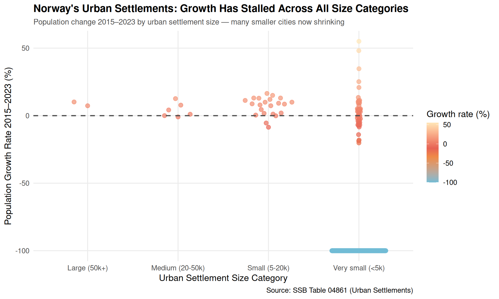
The beeswarm chart reveals a striking pattern: while a few large cities still show modest growth, the majority of urban settlements—especially medium and small ones—have either flatlined or lost population. This is not just a rural story; it’s happening in recognized urban areas.
Some regions buck the trend entirely. Let’s compare the trajectories of Norway’s largest urban areas.
if (!is.null(df_urban)) {
  # Identify major cities by 2023 population
  major_cities <- df_urban |>
    filter(metric == "Bosatte", year == 2023) |>
    arrange(desc(value)) |>
    slice_head(n = 12) |>
    pull(region)

  df_cities <- df_urban |>
    filter(metric == "Bosatte", region %in% major_cities) |>
    arrange(region, year)
}if (!is.null(df_cities)) {
df_slope <- df_cities |>
filter(year %in% c(2015, 2023)) |>
pivot_wider(names_from = year, values_from = value, names_prefix = "pop_") |>
mutate(
growth = pop_2023 - pop_2015,
pct_change = (pop_2023 - pop_2015) / pop_2015 * 100,
direction = ifelse(growth > 0, "Growth", "Decline")
)
p2 <- ggplot(df_slope, aes(x = 1, xend = 2, y = pop_2015, yend = pop_2023)) +
geom_segment(
aes(color = direction),
linewidth = 1.2,
arrow = arrow(length = unit(0.15, "cm"), type = "closed")
) +
geom_text(
aes(x = 0.95, y = pop_2015, label = region),
hjust = 1, size = 3.5, color = "gray20"
) +
geom_text(
aes(x = 2.05, y = pop_2023, label = scales::comma(pop_2023)),
hjust = 0, size = 3.5, color = "gray20"
) +
scale_color_manual(
values = c("Growth" = pal[4], "Decline" = pal[6]),
name = NULL
) +
scale_x_continuous(
limits = c(0.5, 2.5),
breaks = c(1, 2),
labels = c("2015", "2023")
) +
scale_y_continuous(labels = scales::comma) +
labs(
title = "Norway's Major Urban Settlements: Growth Has Become Uneven",
subtitle = "Population trajectories for the 12 largest urban areas — some gained, others plateaued",
x = NULL,
y = "Urban Settlement Population",
caption = "Source: SSB Table 04861 (Urban Settlements)"
) +
theme_minimal(base_size = 13) +
theme(
plot.title = element_text(face = "bold", size = 15),
plot.subtitle = element_text(size = 11, color = "gray30"),
panel.grid.major.x = element_blank(),
panel.grid.minor = element_blank(),
legend.position = "top"
)
print(p2)
}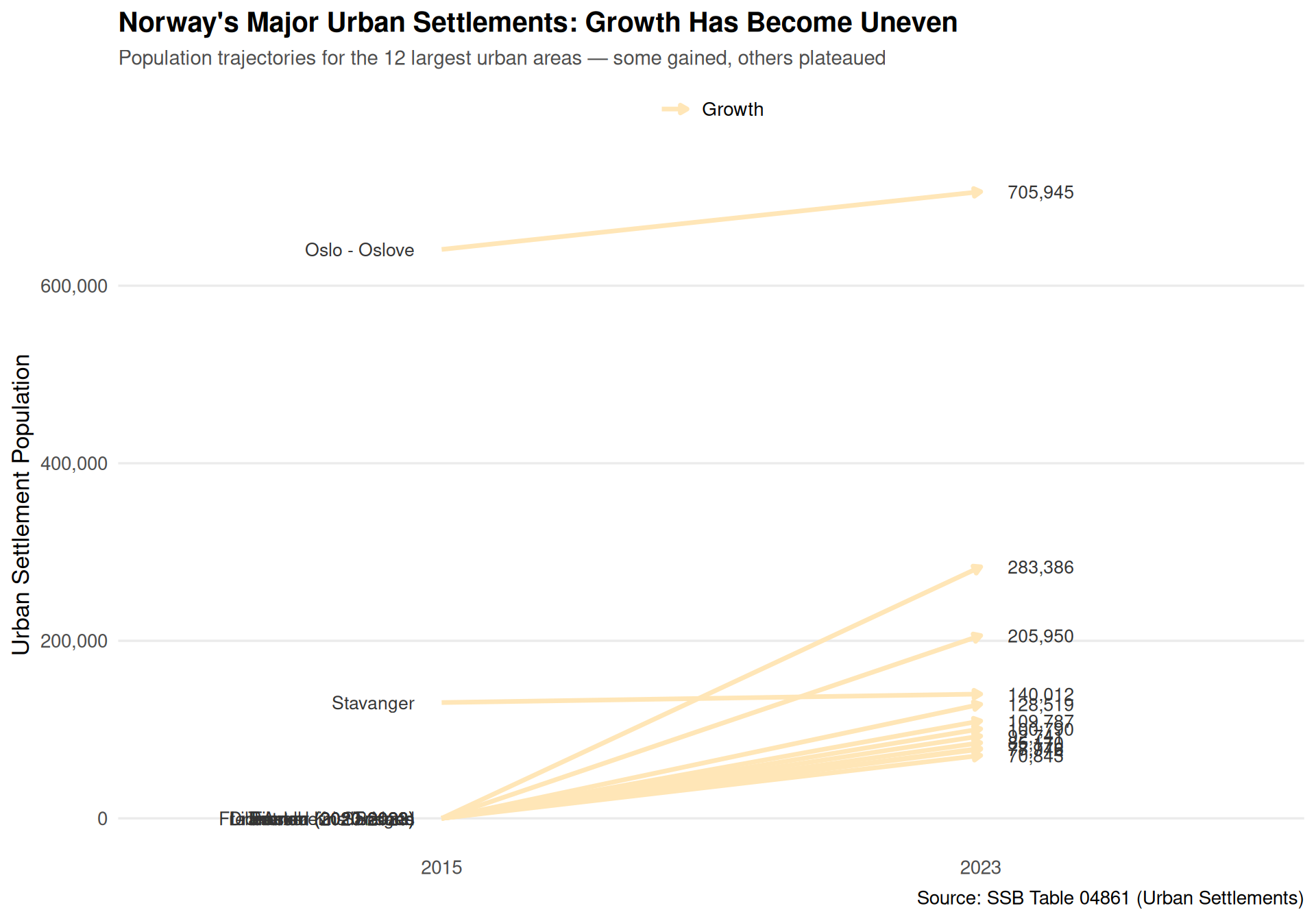
Oslo and a few university cities continue to grow, but the growth rates are nowhere near historical norms. Meanwhile, several formerly dynamic urban centers have essentially frozen in place.
To understand why urban magnetism has weakened, we need to look at Norway’s economic performance. Let’s examine quarterly GDP trends.
df_gdp <- NULL

tryCatch({
  raw <- ApiData(
    "https://data.ssb.no/api/v0/no/table/09190",
    Makrost = c("koh.nrpriv", "koo.nroff", "inv.nrinv"),
    ContentsCode = "VolumEndrSesJust",
    Tid = list(filter = "top", values = 40)
  )

  tmp <- raw[[1]]
  print(names(tmp))

  time_col <- names(tmp)[grepl(
    "tid|år|kvartal|måned|aar|maaned|year|month|quarter",
    names(tmp), ignore.case = TRUE, perl = TRUE
  )][1]
  if (is.na(time_col)) time_col <- names(tmp)[length(names(tmp)) - 1L]

  value_col <- names(tmp)[vapply(tmp, is.numeric, logical(1L))][1]
  if (is.na(value_col)) value_col <- names(tmp)[length(names(tmp))]

  sector_col <- names(tmp)[grepl("makrost|sektor|sector", names(tmp), ignore.case = TRUE)][1]

  df_gdp <- tmp |>
    mutate(
      value = as.numeric(.data[[value_col]]),
      time_str = .data[[time_col]],
      date = lubridate::yq(sub("K", " Q", time_str)),
      sector = .data[[sector_col]]
    ) |>
    filter(!is.na(value), !is.na(date))

}, error = function(e) message("GDP data fetch failed: ", e$message))if (!is.null(df_gdp)) {
p3 <- df_gdp |>
ggplot(aes(x = date, y = value, fill = sector)) +
geom_area(alpha = 0.7, position = "identity") +
geom_hline(yintercept = 0, linetype = "dashed", color = "gray30", linewidth = 0.8) +
scale_fill_manual(
values = c(pal[1], pal[4], pal[6]),
name = "GDP Component",
labels = c(
"koh.nrpriv" = "Household consumption",
"koo.nroff" = "Government consumption",
"inv.nrinv" = "Total investment"
)
) +
scale_x_date(date_breaks = "2 years", date_labels = "%Y") +
labs(
title = "Norway's Economic Growth Momentum Has Evaporated Since 2022",
subtitle = "Quarterly volume change from previous quarter, seasonally adjusted — investment collapsed, consumption stagnated",
x = NULL,
y = "Volume Change from Previous Quarter (%)",
caption = "Source: SSB Table 09190 (Quarterly GDP)"
) +
theme_minimal(base_size = 13) +
theme(
plot.title = element_text(face = "bold", size = 15),
plot.subtitle = element_text(size = 11, color = "gray30"),
panel.grid.minor = element_blank(),
legend.position = "top"
)
print(p3)
}The GDP chart tells the story: Norway’s economy has been sputtering. Investment collapsed in 2024–2025, household consumption barely grew, and government spending couldn’t compensate. Without economic dynamism, cities lose their pull.
Finally, let’s examine the labor market itself. Has the nature of work changed in ways that make urban concentration less necessary?
df_labor <- NULL

tryCatch({
  raw <- ApiData(
    "https://data.ssb.no/api/v0/no/table/13760",
    Kjonn = "0",
    Alder = "15-74",
    Justering = "S",
    ContentsCode = c("Sysselsatte", "Arbeidsledige", "ArbledProsArbstyrk"),
    Tid = list(filter = "top", values = 60)
  )

  tmp <- raw[[1]]
  print(names(tmp))

  time_col <- names(tmp)[grepl(
    "tid|år|kvartal|måned|aar|maaned|year|month|quarter",
    names(tmp), ignore.case = TRUE, perl = TRUE
  )][1]
  if (is.na(time_col)) time_col <- names(tmp)[length(names(tmp)) - 1L]

  value_col <- names(tmp)[vapply(tmp, is.numeric, logical(1L))][1]
  if (is.na(value_col)) value_col <- names(tmp)[length(names(tmp))]

  content_col <- names(tmp)[grepl("statistikk|contents|innhold", names(tmp), ignore.case = TRUE)][1]

  df_labor <- tmp |>
    mutate(
      value = as.numeric(.data[[value_col]]),
      time_str = .data[[time_col]],
      date = lubridate::ym(sub("M", "-", time_str)),
      metric = .data[[content_col]]
    ) |>
    filter(!is.na(value), !is.na(date))

}, error = function(e) message("Labor data fetch failed: ", e$message))
[1] "kjønn" "alder" "type justering"
[4] "statistikkvariabel" "måned" "value" if (!is.null(df_labor)) {
# Create time periods for alluvial-style comparison
df_periods <- df_labor |>
mutate(
period = case_when(
year(date) <= 2019 ~ "Pre-pandemic",
year(date) >= 2020 & year(date) <= 2021 ~ "Pandemic",
year(date) >= 2022 & year(date) <= 2023 ~ "Recovery",
TRUE ~ "Current"
)
) |>
filter(metric %in% c("Sysselsatte", "Arbeidsledige")) |>
group_by(period, metric) |>
summarise(avg_value = mean(value, na.rm = TRUE), .groups = "drop") |>
filter(!is.na(period))
p4 <- df_periods |>
ggplot(aes(x = period, y = avg_value, group = metric, color = metric)) +
geom_line(linewidth = 1.5, alpha = 0.8) +
geom_point(size = 4) +
scale_color_manual(
values = c("Sysselsatte" = pal[4], "Arbeidsledige" = pal[6]),
name = "Labor Market Indicator",
labels = c("Sysselsatte" = "Employed (1000s)", "Arbeidsledige" = "Unemployed (1000s)")
) +
scale_x_discrete(limits = c("Pre-pandemic", "Pandemic", "Recovery", "Current")) +
scale_y_continuous(labels = scales::comma) +
labs(
title = "Norway's Labor Market: Employment High, Unemployment Low — But Cities Still Losing People",
subtitle = "Average monthly employment and unemployment by period, seasonally adjusted — tight labor market hasn't prevented urban stagnation",
x = NULL,
y = "Number of People (thousands)",
caption = "Source: SSB Table 13760 (Labour Force Survey)"
) +
theme_minimal(base_size = 13) +
theme(
plot.title = element_text(face = "bold", size = 15),
plot.subtitle = element_text(size = 11, color = "gray30"),
panel.grid.minor = element_blank(),
legend.position = "top"
)
print(p4)
}
Paradoxically, Norway’s labor market remains remarkably strong: employment is high, unemployment is low. Yet urban areas aren’t capturing the benefits. The explanation likely lies in remote work and distributed employment—people can now work for urban employers without living in urban settlements.
Urban growth has collapsed: Between 2015 and 2023, many Norwegian urban settlements saw zero or negative population growth—a sharp reversal from previous decades.
Size no longer guarantees growth: Even medium-sized cities (20,000–50,000 residents) have stagnated, while some small settlements are shrinking rapidly.
Economic weakness accelerated the trend: Norway’s GDP growth evaporated after 2022, with investment and consumption both flat, removing the economic pull that once drove urbanization.
The labor market paradox: Despite low unemployment and high employment, cities aren’t attracting people—suggesting remote work and geographic flexibility have fundamentally changed settlement patterns.
Oslo still grows, but slowly: Even Norway’s capital and largest urban area is growing far more slowly than historical trends would predict.
The plateau in urban growth marks a fundamental shift in Norwegian society. For decades, policymakers could assume that cities would continue expanding, justifying infrastructure investments, housing development, and service concentration. That assumption no longer holds.
The implications ripple across multiple domains: housing markets will likely remain soft in many urban areas, municipal finances will struggle without population-driven revenue growth, and regional development strategies will need rethinking. Meanwhile, rural and small-town Norway—written off by many analysts—may be experiencing a quiet renaissance as remote work makes location less binding.
The question now is whether this represents a temporary pause or a permanent restructuring. If economic growth returns, will cities regain their magnetic pull? Or has the pandemic-era discovery of geographic flexibility created a lasting preference for smaller settlements and lower density? Norway’s next decade of urban data will tell us which future we’re heading toward.