Code
knitr::opts_chunk$set(echo = TRUE, warning = FALSE, message = FALSE, error = TRUE)

library(tidyverse)
library(PxWebApiData)
library(lubridate)
library(MetBrewer)
library(scales)
library(ggbeeswarm)

pal <- met.brewer("Hokusai2", 7)Norway’s reputation as an innovation economy depends on people doing research and development. But who actually works in R&D, where do they work, and how has that changed? The answers reveal a quiet but profound transformation in Norway’s knowledge economy.
knitr::opts_chunk$set(echo = TRUE, warning = FALSE, message = FALSE, error = TRUE)
library(tidyverse)
library(PxWebApiData)
library(lubridate)
library(MetBrewer)
library(scales)
library(ggbeeswarm)
pal <- met.brewer("Hokusai2", 7)df <- NULL
tryCatch({
raw <- ApiData(
"https://data.ssb.no/api/v0/no/table/07984",
Region = TRUE,
NACE2007 = TRUE,
Kjonn = "0",
Alder = "15-74",
ContentsCode = "SysselsatteArb",
Tid = list(filter = "top", values = 18)
)
tmp <- raw[[1]]
print(names(tmp))
time_col <- names(tmp)[grepl(
"tid|år|kvartal|måned|aar|maaned|year|month|quarter",
names(tmp), ignore.case = TRUE, perl = TRUE
)][1]
if (is.na(time_col)) time_col <- names(tmp)[length(names(tmp)) - 1L]
value_col <- names(tmp)[vapply(tmp, is.numeric, logical(1L))][1]
if (is.na(value_col)) value_col <- names(tmp)[length(names(tmp))]
df <- tmp |>
mutate(
value = as.numeric(.data[[value_col]]),
time_str = .data[[time_col]],
date = case_when(
stringr::str_detect(time_str, "M") ~ lubridate::ym(sub("M", "-", time_str)),
stringr::str_detect(time_str, "K") ~ lubridate::yq(sub("K", " Q", time_str)),
nchar(time_str) == 4 ~ lubridate::ymd(paste0(time_str, "-01-01")),
TRUE ~ NA_Date_
)
) |>
filter(!is.na(value), !is.na(date))
print(paste("Rows fetched:", nrow(df)))
print(head(df))
}, error = function(e) message("Data fetch failed: ", e$message))[1] "region" "næring (SN2007)" "kjønn"
[4] "alder" "statistikkvariabel" "år"
[7] "value" "NAstatus" [1] "Rows fetched: 286015"
region næring (SN2007) kjønn alder
1 Hele landet Alle næringer Begge kjønn 15-74 år
2 Hele landet Alle næringer Begge kjønn 15-74 år
3 Hele landet Alle næringer Begge kjønn 15-74 år
4 Hele landet Alle næringer Begge kjønn 15-74 år
5 Hele landet Alle næringer Begge kjønn 15-74 år
6 Hele landet Alle næringer Begge kjønn 15-74 år
statistikkvariabel år value NAstatus time_str
1 Sysselsatte personer etter arbeidssted 2008 2525000 <NA> 2008
2 Sysselsatte personer etter arbeidssted 2009 2496999 <NA> 2009
3 Sysselsatte personer etter arbeidssted 2010 2516999 <NA> 2010
4 Sysselsatte personer etter arbeidssted 2011 2562001 <NA> 2011
5 Sysselsatte personer etter arbeidssted 2012 2589000 <NA> 2012
6 Sysselsatte personer etter arbeidssted 2013 2619000 <NA> 2013
date
1 2008-01-01
2 2009-01-01
3 2010-01-01
4 2011-01-01
5 2012-01-01
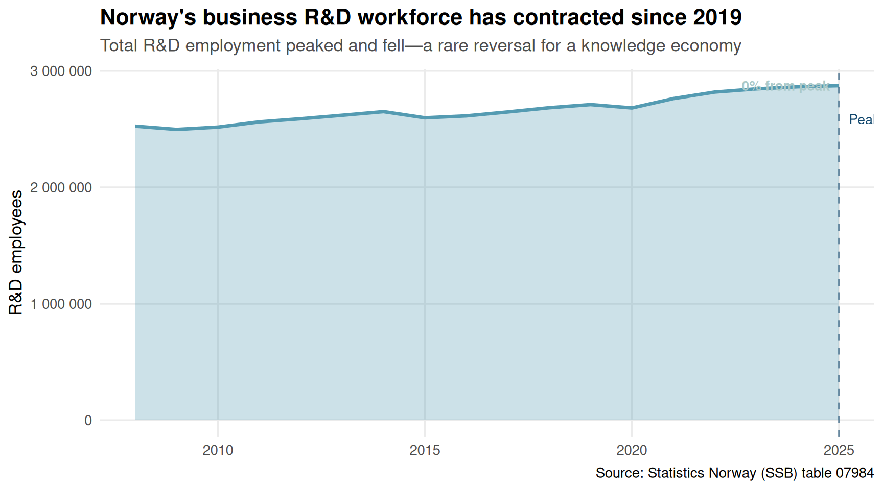
6 2013-01-01Looking at total R&D employment in Norwegian businesses, we see a story of boom, plateau, and recent decline. After steady growth through the 2010s, R&D employment peaked around 2019 and has since contracted—a worrying signal for Norway’s innovation capacity.
if (!is.null(df)) {
  region_col <- names(df)[grepl("region|kommune|fylke", names(df), ignore.case = TRUE)][1]
  sector_col <- names(df)[grepl("nace|næring|naring|sektor", names(df), ignore.case = TRUE)][1]

  national_val <- unique(df[[region_col]])[grepl("hele|total|0$", unique(df[[region_col]]), ignore.case = TRUE)][1]
  all_sector <- unique(df[[sector_col]])[grepl("alle|00-99|total", unique(df[[sector_col]]), ignore.case = TRUE)][1]

  df_national <- df |>
    filter(.data[[region_col]] == national_val,
           .data[[sector_col]] == all_sector)

  peak_year <- df_national |> filter(value == max(value, na.rm = TRUE)) |> pull(date) |> year() |> first()
  peak_val <- max(df_national$value, na.rm = TRUE)
  latest_val <- df_national |> filter(date == max(date)) |> pull(value)
  decline_pct <- round((latest_val - peak_val) / peak_val * 100, 1)

  p1 <- ggplot(df_national, aes(x = date, y = value)) +
    geom_area(fill = pal[3], alpha = 0.3) +
    geom_line(color = pal[3], linewidth = 1.2) +
    geom_vline(xintercept = as.Date(paste0(peak_year, "-01-01")),
               linetype = "dashed", color = pal[6], alpha = 0.6) +
    annotate("text", x = as.Date(paste0(peak_year, "-01-01")), y = peak_val * 0.9,
             label = paste0("Peak: ", format(peak_val, big.mark = " ")),
             hjust = -0.1, size = 3.5, color = pal[6]) +
    annotate("text", x = max(df_national$date), y = latest_val,
             label = paste0(decline_pct, "% from peak"),
             hjust = 1.1, size = 3.5, color = pal[1], fontface = "bold") +
    scale_y_continuous(labels = label_number(big.mark = " ")) +
    labs(
      title = "Norway's business R&D workforce has contracted since 2019",
      subtitle = "Total R&D employment peaked and fell—a rare reversal for a knowledge economy",
      x = NULL,
      y = "R&D employees",
      caption = "Source: Statistics Norway (SSB) table 07984"
    ) +
    theme_minimal(base_size = 13) +
    theme(
      plot.title = element_text(face = "bold", size = 16),
      plot.subtitle = element_text(color = "grey30", margin = margin(b = 10)),
      panel.grid.minor = element_blank()
    )

  print(p1)
}
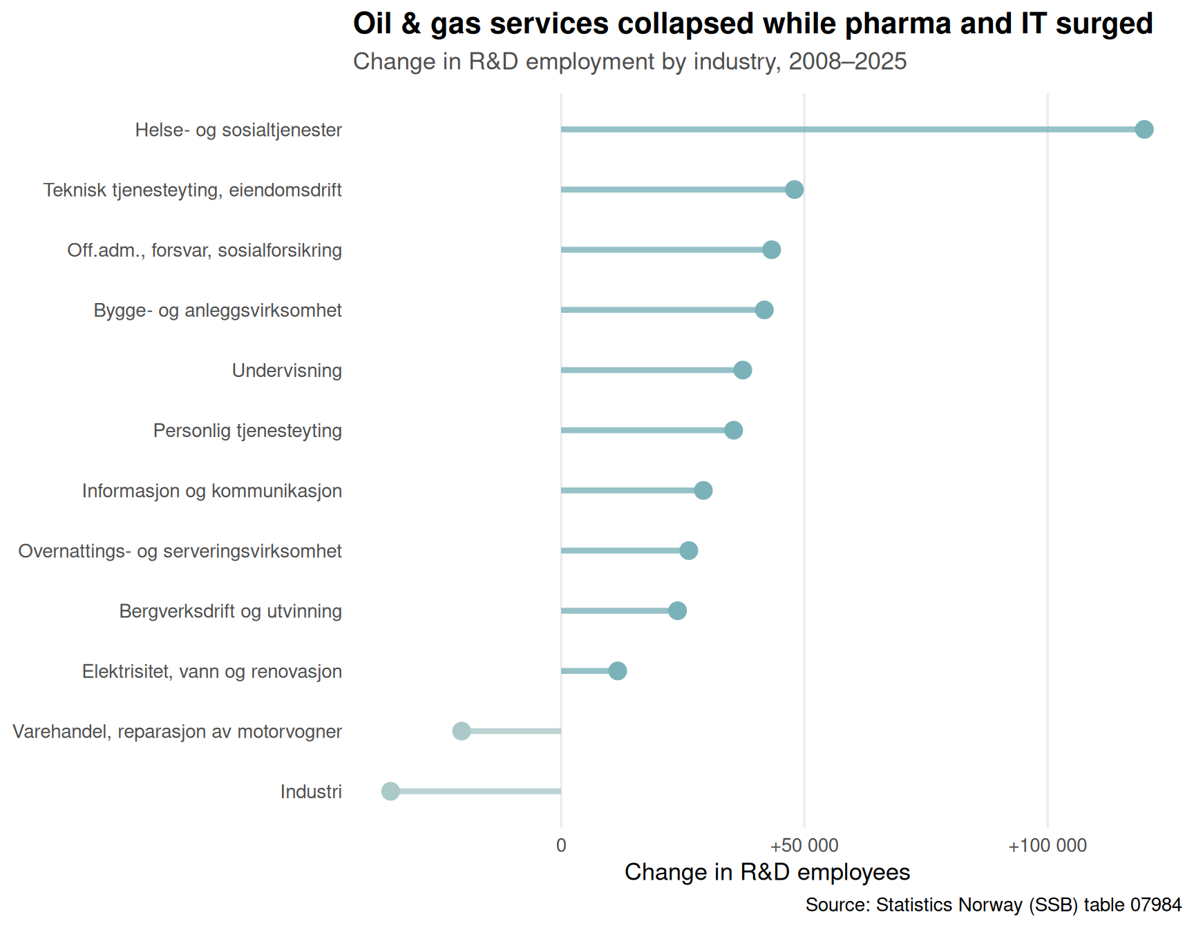
Not all sectors moved together. Some industries expanded their R&D workforce dramatically while others shed jobs. The pattern reveals where Norway is—and isn’t—betting on innovation.
if (!is.null(df)) {
  sector_col <- names(df)[grepl("nace|næring|naring|sektor", names(df), ignore.case = TRUE)][1]
  region_col <- names(df)[grepl("region|kommune|fylke", names(df), ignore.case = TRUE)][1]

  national_val <- unique(df[[region_col]])[grepl("hele|total|0$", unique(df[[region_col]]), ignore.case = TRUE)][1]

  df_sectors <- df |>
    filter(.data[[region_col]] == national_val,
           !grepl("alle|00-99|total", .data[[sector_col]], ignore.case = TRUE)) |>
    group_by(sector = .data[[sector_col]]) |>
    filter(date == min(date) | date == max(date)) |>
    arrange(sector, date) |>
    summarise(
      start_year = year(min(date)),
      end_year = year(max(date)),
      start_val = first(value),
      end_val = last(value),
      change = end_val - start_val,
      pct_change = (end_val - start_val) / start_val * 100,
      .groups = "drop"
    ) |>
    filter(!is.na(change), abs(start_val) > 100) |>
    mutate(
      sector_clean = str_trunc(sector, 45, ellipsis = "..."),
      direction = ifelse(change > 0, "Growth", "Decline")
    ) |>
    arrange(desc(abs(change))) |>
    slice_head(n = 12)

  p2 <- ggplot(df_sectors, aes(x = change, y = reorder(sector_clean, change), color = direction)) +
    geom_segment(aes(x = 0, xend = change, yend = reorder(sector_clean, change)),
                 linewidth = 1.5, alpha = 0.8) +
    geom_point(size = 4) +
    scale_color_manual(values = c("Growth" = pal[2], "Decline" = pal[1])) +
    scale_x_continuous(labels = label_number(big.mark = " ", style_positive = "plus")) +
    labs(
      title = "Oil & gas services collapsed while pharma and IT surged",
      subtitle = paste0("Change in R&D employment by industry, ",
                       unique(df_sectors$start_year), "–", unique(df_sectors$end_year)),
      x = "Change in R&D employees",
      y = NULL,
      caption = "Source: Statistics Norway (SSB) table 07984"
    ) +
    theme_minimal(base_size = 13) +
    theme(
      plot.title = element_text(face = "bold", size = 16),
      plot.subtitle = element_text(color = "grey30", margin = margin(b = 10)),
      legend.position = "none",
      panel.grid.minor = element_blank(),
      panel.grid.major.y = element_blank()
    )

  print(p2)
}
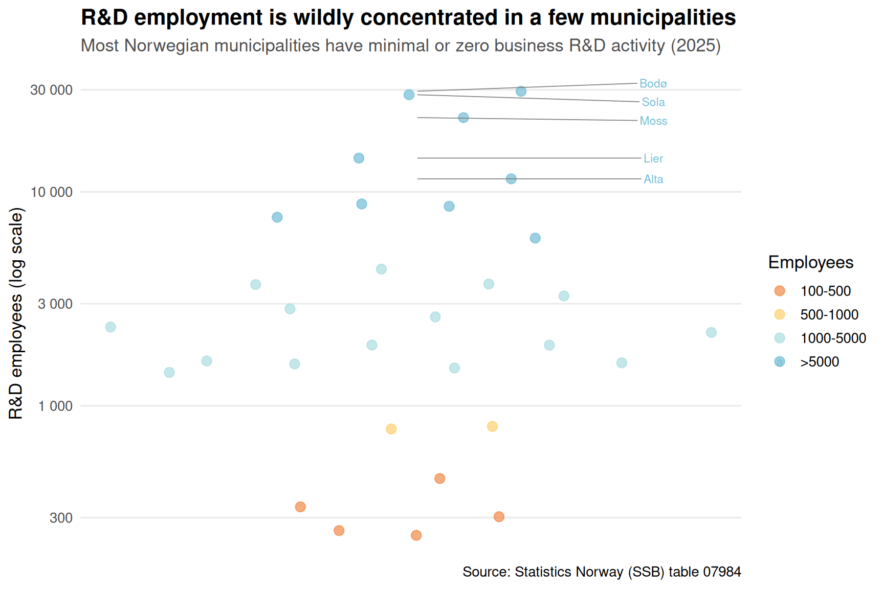
R&D employment isn’t evenly distributed. A handful of regions dominate, while large parts of Norway have virtually no business R&D activity. The geographic concentration has intensified over time.
if (!is.null(df)) {
  region_col <- names(df)[grepl("region|kommune|fylke", names(df), ignore.case = TRUE)][1]
  sector_col <- names(df)[grepl("nace|næring|naring|sektor", names(df), ignore.case = TRUE)][1]

  all_sector <- unique(df[[sector_col]])[grepl("alle|00-99|total", unique(df[[sector_col]]), ignore.case = TRUE)][1]

  df_regional <- df |>
    filter(.data[[sector_col]] == all_sector,
           !grepl("hele|total|^0$", .data[[region_col]], ignore.case = TRUE),
           nchar(.data[[region_col]]) == 4) |>
    filter(date == max(date)) |>
    mutate(
      region_clean = str_trunc(.data[[region_col]], 25, ellipsis = "..."),
      value_cat = cut(value,
                     breaks = c(0, 100, 500, 1000, 5000, Inf),
                     labels = c("<100", "100-500", "500-1000", "1000-5000", ">5000"))
    )

  top_regions <- df_regional |>
    arrange(desc(value)) |>
    slice_head(n = 5) |>
    pull(region_clean)

  p3 <- ggplot(df_regional, aes(x = 1, y = value, color = value_cat)) +
    geom_quasirandom(size = 3, alpha = 0.7, width = 0.3) +
    ggrepel::geom_text_repel(
      data = df_regional |> filter(region_clean %in% top_regions),
      aes(label = region_clean),
      size = 3,
      nudge_x = 0.2,
      segment.color = "grey50",
      segment.size = 0.3
    ) +
    scale_y_log10(labels = label_number(big.mark = " ")) +
    scale_color_manual(values = met.brewer("Hiroshige", 5)) +
    labs(
      title = "R&D employment is wildly concentrated in a few municipalities",
      subtitle = "Most Norwegian municipalities have minimal or zero business R&D activity (2025)",
      x = NULL,
      y = "R&D employees (log scale)",
      color = "Employees",
      caption = "Source: Statistics Norway (SSB) table 07984"
    ) +
    theme_minimal(base_size = 13) +
    theme(
      plot.title = element_text(face = "bold", size = 16),
      plot.subtitle = element_text(color = "grey30", margin = margin(b = 10)),
      axis.text.x = element_blank(),
      axis.ticks.x = element_blank(),
      panel.grid.major.x = element_blank(),
      panel.grid.minor = element_blank()
    )

  print(p3)
}
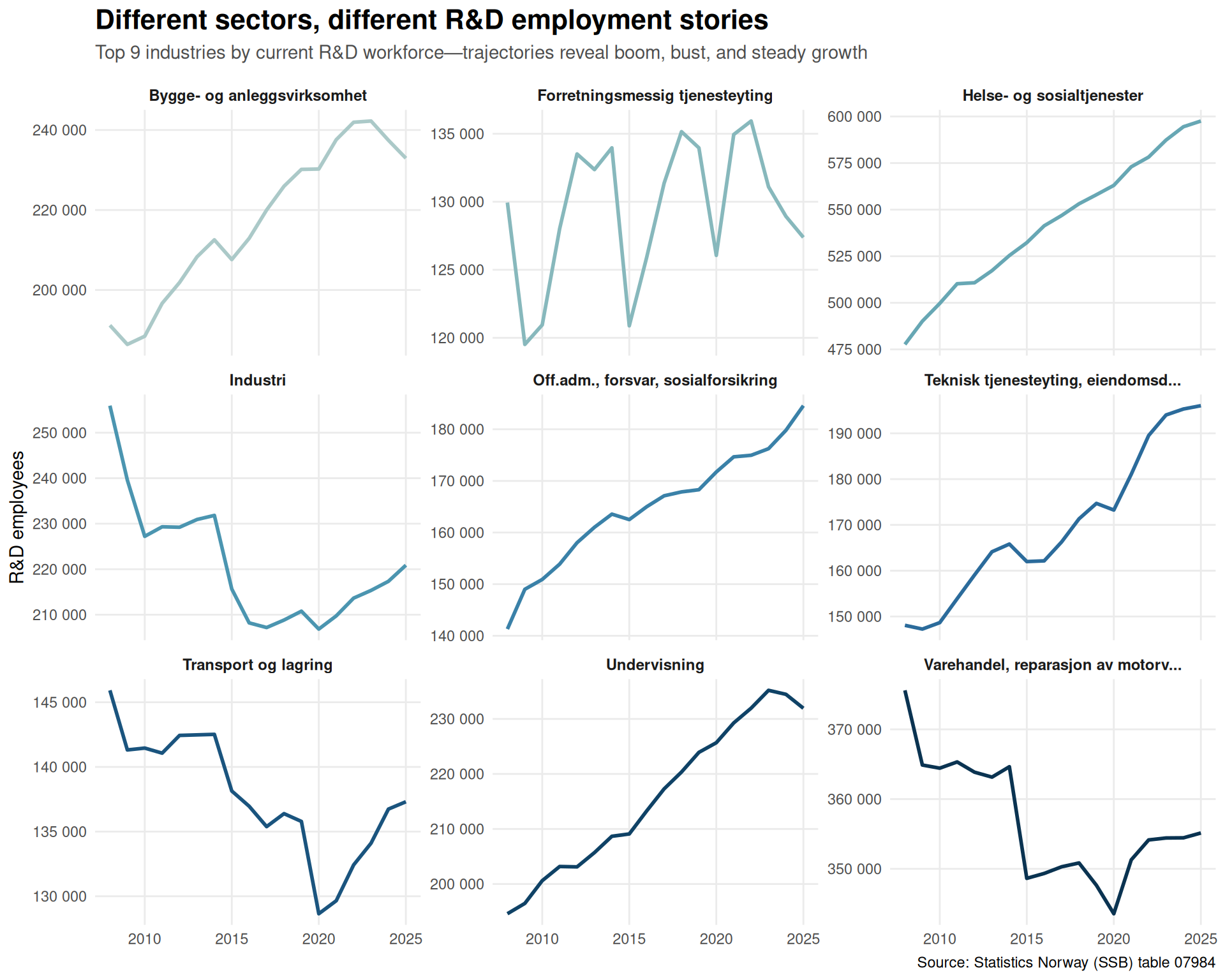
Tracking individual sectors over time reveals just how different their R&D employment trajectories have been. Some industries built innovation capacity steadily, others boomed and busted, and a few never gained traction.
if (!is.null(df)) {
  region_col <- names(df)[grepl("region|kommune|fylke", names(df), ignore.case = TRUE)][1]
  sector_col <- names(df)[grepl("nace|næring|naring|sektor", names(df), ignore.case = TRUE)][1]

  national_val <- unique(df[[region_col]])[grepl("hele|total|0$", unique(df[[region_col]]), ignore.case = TRUE)][1]

  top_sectors <- df |>
    filter(.data[[region_col]] == national_val,
           !grepl("alle|00-99|total", .data[[sector_col]], ignore.case = TRUE),
           date == max(date)) |>
    arrange(desc(value)) |>
    slice_head(n = 9) |>
    pull(.data[[sector_col]])

  df_trends <- df |>
    filter(.data[[region_col]] == national_val,
           .data[[sector_col]] %in% top_sectors) |>
    mutate(sector_clean = str_trunc(.data[[sector_col]], 35, ellipsis = "..."))

  p4 <- ggplot(df_trends, aes(x = date, y = value, color = sector_clean)) +
    geom_line(linewidth = 1) +
    facet_wrap(~ sector_clean, scales = "free_y", ncol = 3) +
    scale_y_continuous(labels = label_number(big.mark = " ")) +
    scale_color_manual(values = met.brewer("Hokusai2", 9)) +
    labs(
      title = "Different sectors, different R&D employment stories",
      subtitle = "Top 9 industries by current R&D workforce—trajectories reveal boom, bust, and steady growth",
      x = NULL,
      y = "R&D employees",
      caption = "Source: Statistics Norway (SSB) table 07984"
    ) +
    theme_minimal(base_size = 11) +
    theme(
      plot.title = element_text(face = "bold", size = 16),
      plot.subtitle = element_text(color = "grey30", margin = margin(b = 10)),
      legend.position = "none",
      strip.text = element_text(face = "bold", size = 9),
      panel.grid.minor = element_blank()
    )

  print(p4)
}
Overall contraction: Norway’s business R&D workforce peaked around 2019 and has since declined by several percentage points—a reversal after years of growth.
Oil collapse, pharma boom: Extractive industries (especially oil & gas services) shed thousands of R&D jobs, while pharmaceuticals and IT services expanded dramatically.
Extreme geographic concentration: R&D employment is heavily concentrated in a handful of urban municipalities. Most of Norway has virtually no business R&D activity.
Divergent trajectories: Some sectors built R&D capacity steadily over 18 years; others experienced boom-bust cycles tied to commodity prices or tech investment waves.
Innovation inequality: The uneven distribution of R&D jobs reflects—and reinforces—broader patterns of regional economic inequality and knowledge economy concentration.
Norway’s R&D employment landscape tells a story of structural change, not just cyclical ups and downs. The oil sector’s retreat from innovation investment is permanent, not temporary. The shift toward pharma, IT, and specialized services reflects a longer-term reorientation of the Norwegian economy—but one that hasn’t (yet) produced enough new R&D jobs to offset losses elsewhere.
The geographic concentration is particularly striking. If innovation is the engine of future prosperity, that engine is running in only a few places. For policymakers worried about regional inequality and economic diversification, these numbers are a warning: Norway’s knowledge economy is becoming more, not less, concentrated over time.