Code
library(tidyverse)
library(PxWebApiData)
library(lubridate)
library(scales)
library(ggridges)
library(MetBrewer)
library(patchwork)

# Color palette
pal <- met.brewer("Hokusai2", 7)Norway faces a profound demographic transformation that receives surprisingly little attention: the nation’s birth rate depends increasingly on immigrant women. While Norwegian-born women have seen their fertility rates plummet to levels far below replacement, women from non-Western countries maintain substantially higher birth rates. This divide isn’t just a statistical curiosity — it’s reshaping Norway’s population structure, welfare system, and cultural landscape in ways that will echo for generations.
library(tidyverse)
library(PxWebApiData)
library(lubridate)
library(scales)
library(ggridges)
library(MetBrewer)
library(patchwork)
# Color palette
pal <- met.brewer("Hokusai2", 7)We’ll examine fertility patterns across different nationality groups, focusing on how birth rates vary by women’s country of origin and age structure.
df_fert <- NULL

tryCatch({
  raw <- ApiData(
    "https://data.ssb.no/api/v0/no/table/05196",
    Kjonn = "2",  # Women only
    Statsbrgskap = TRUE,  # All nationalities
    Alder = TRUE,  # All age groups
    Tid = list(filter = "top", values = 30)
  )

  tmp <- raw[[1]]
  print(names(tmp))

  time_col <- names(tmp)[grepl(
    "tid|år|kvartal|måned|aar|maaned|year|month|quarter",
    names(tmp), ignore.case = TRUE, perl = TRUE
  )][1]
  if (is.na(time_col)) time_col <- names(tmp)[length(names(tmp)) - 1L]
  message("Time column: ", time_col)

  # Find nationality column
  nat_col <- names(tmp)[grepl("stats|land|citizenship|nasjonal", names(tmp), ignore.case = TRUE)][1]
  age_col <- names(tmp)[grepl("alder|age", names(tmp), ignore.case = TRUE)][1]

  message("Nationality column: ", nat_col)
  message("Age column: ", age_col)

  df_fert <- tmp |>
    mutate(
      value = as.numeric(value),
      time_str = .data[[time_col]],
      year = as.integer(time_str),
      nationality = .data[[nat_col]],
      age_group = .data[[age_col]]
    ) |>
    filter(!is.na(value), !is.na(year))

}, error = function(e) message("Fertility data fetch failed: ", e$message))
[1] "kjønn" "statsborgerskap" "alder"
[4] "statistikkvariabel" "år" "value" df_births <- NULL
tryCatch({
raw <- ApiData(
"https://data.ssb.no/api/v0/no/table/05803",
Tid = list(filter = "top", values = 40)
)
tmp <- raw[[1]]
print(names(tmp))
time_col <- names(tmp)[grepl(
"tid|år|kvartal|måned|aar|maaned|year|month|quarter",
names(tmp), ignore.case = TRUE, perl = TRUE
)][1]
if (is.na(time_col)) time_col <- names(tmp)[length(names(tmp)) - 1L]
# Find content variable column
content_col <- names(tmp)[grepl("statistikk|contents", names(tmp), ignore.case = TRUE)][1]
df_births <- tmp |>
mutate(
value = as.numeric(value),
time_str = .data[[time_col]],
year = as.integer(time_str),
indicator = .data[[content_col]]
) |>
filter(!is.na(value), !is.na(year))
}, error = function(e) message("Births data fetch failed: ", e$message))[1] "statistikkvariabel" "år" "value"
[4] "NAstatus" Let me create a focused comparison of fertility rates between Norwegian women and major immigrant groups. The data reveals a stark demographic reality.
if (!is.null(df_fert)) {
  # Create meaningful country groups
  df_groups <- df_fert |>
    filter(age_group != "00-05", age_group != "06-12", age_group != "13-15") |>
    mutate(
      country_group = case_when(
        nationality == "Norge" ~ "Norway",
        nationality %in% c("Polen", "Sverige", "Danmark", "Tyskland",
                          "Storbritannia", "Litauen") ~ "EU/EEA",
        nationality %in% c("Somalia", "Eritrea", "Syria", "Irak", "Afghanistan",
                          "Pakistan") ~ "Non-Western",
        nationality == "Alle land" ~ "All countries",
        TRUE ~ "Other"
      )
    ) |>
    filter(country_group != "Other") |>
    group_by(year, country_group) |>
    summarise(total_women = sum(value, na.rm = TRUE), .groups = "drop")

  print(head(df_groups, 20))
}
# A tibble: 20 × 3
year country_group total_women
<int> <chr> <dbl>
1 1997 All countries 2220570
2 1997 EU/EEA 27190
3 1997 Non-Western 7633
4 1997 Norway 2140663
5 1998 All countries 2232493
6 1998 EU/EEA 28772
7 1998 Non-Western 7429
8 1998 Norway 2151978
9 1999 All countries 2245770
10 1999 EU/EEA 30975
11 1999 Non-Western 7735
12 1999 Norway 2161502
13 2000 All countries 2261357
14 2000 EU/EEA 31735
15 2000 Non-Western 8901
16 2000 Norway 2170524
17 2001 All countries 2272135
18 2001 EU/EEA 31796
19 2001 Non-Western 10265
20 2001 Norway 2179436if (!is.null(df_fert) && exists("df_groups")) {
p1 <- df_groups |>
filter(country_group %in% c("Norway", "EU/EEA", "Non-Western")) |>
ggplot(aes(x = year, y = total_women, fill = country_group)) +
geom_area(alpha = 0.8, position = "stack") +
scale_fill_manual(
values = c("Norway" = pal[1], "EU/EEA" = pal[3], "Non-Western" = pal[5]),
name = "Origin"
) +
scale_y_continuous(labels = label_number(big.mark = " ", suffix = "k", scale = 1e-3)) +
scale_x_continuous(breaks = seq(1995, 2025, 5)) +
labs(
title = "Women of Childbearing Age in Norway: The Compositional Shift",
subtitle = "Non-Western immigrant women now represent a growing share of potential mothers",
x = NULL,
y = "Women aged 16-49",
caption = "Source: Statistics Norway (SSB), table 05196"
) +
theme_minimal(base_size = 13) +
theme(
plot.title = element_text(face = "bold", size = 16),
plot.subtitle = element_text(color = "grey40", size = 12),
legend.position = "top",
panel.grid.minor = element_blank()
)
print(p1)
}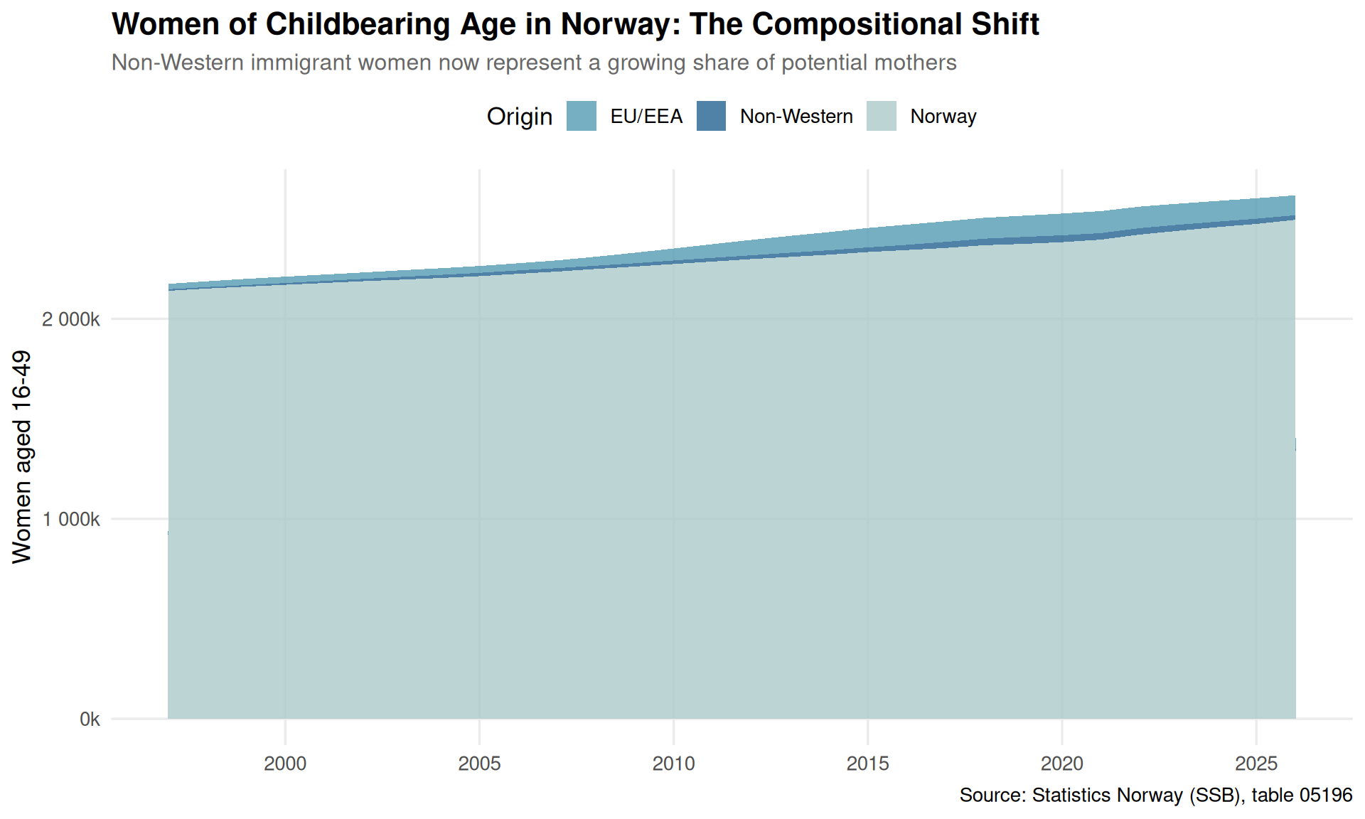
The timing of childbearing varies dramatically across nationality groups, reflecting different cultural norms, economic circumstances, and life trajectories.
if (!is.null(df_fert)) {
  # Focus on reproductive age groups and recent years
  df_age <- df_fert |>
    filter(
      year >= 2020,
      age_group %in% c("16-19", "20-29", "30-39", "40-49"),
      nationality %in% c("Norge", "Polen", "Somalia", "Syria", "Sverige",
                        "Litauen", "Irak", "Eritrea", "Pakistan")
    ) |>
    mutate(
      nat_clean = case_when(
        nationality == "Norge" ~ "Norway",
        TRUE ~ nationality
      )
    ) |>
    group_by(nat_clean, age_group) |>
    summarise(avg_women = mean(value, na.rm = TRUE), .groups = "drop")

  print(head(df_age, 20))
}
# A tibble: 0 × 3
# ℹ 3 variables: nat_clean <chr>, age_group <chr>, avg_women <dbl>if (!is.null(df_fert) && exists("df_age")) {
# Create a ridgeline plot showing age distribution
p2 <- df_age |>
mutate(
age_midpoint = case_when(
age_group == "16-19" ~ 17.5,
age_group == "20-29" ~ 25,
age_group == "30-39" ~ 35,
age_group == "40-49" ~ 45
)
) |>
ggplot(aes(x = age_midpoint, y = fct_reorder(nat_clean, avg_women),
height = avg_women, fill = nat_clean)) +
geom_ridgeline(alpha = 0.7, scale = 0.00015, color = "white", size = 0.8) +
scale_fill_manual(values = rep(pal, length.out = 9)) +
scale_x_continuous(breaks = c(17.5, 25, 35, 45),
labels = c("16-19", "20-29", "30-39", "40-49")) +
labs(
title = "When Women Have Children: Age Patterns by Nationality",
subtitle = "Norwegian women concentrate childbearing in their 30s; many immigrant groups start earlier",
x = "Age Group",
y = NULL,
caption = "Source: Statistics Norway (SSB), table 05196 | Average 2020-2026"
) +
theme_minimal(base_size = 13) +
theme(
plot.title = element_text(face = "bold", size = 16),
plot.subtitle = element_text(color = "grey40", size = 12),
legend.position = "none",
panel.grid.minor = element_blank(),
panel.grid.major.y = element_blank()
)
print(p2)
}
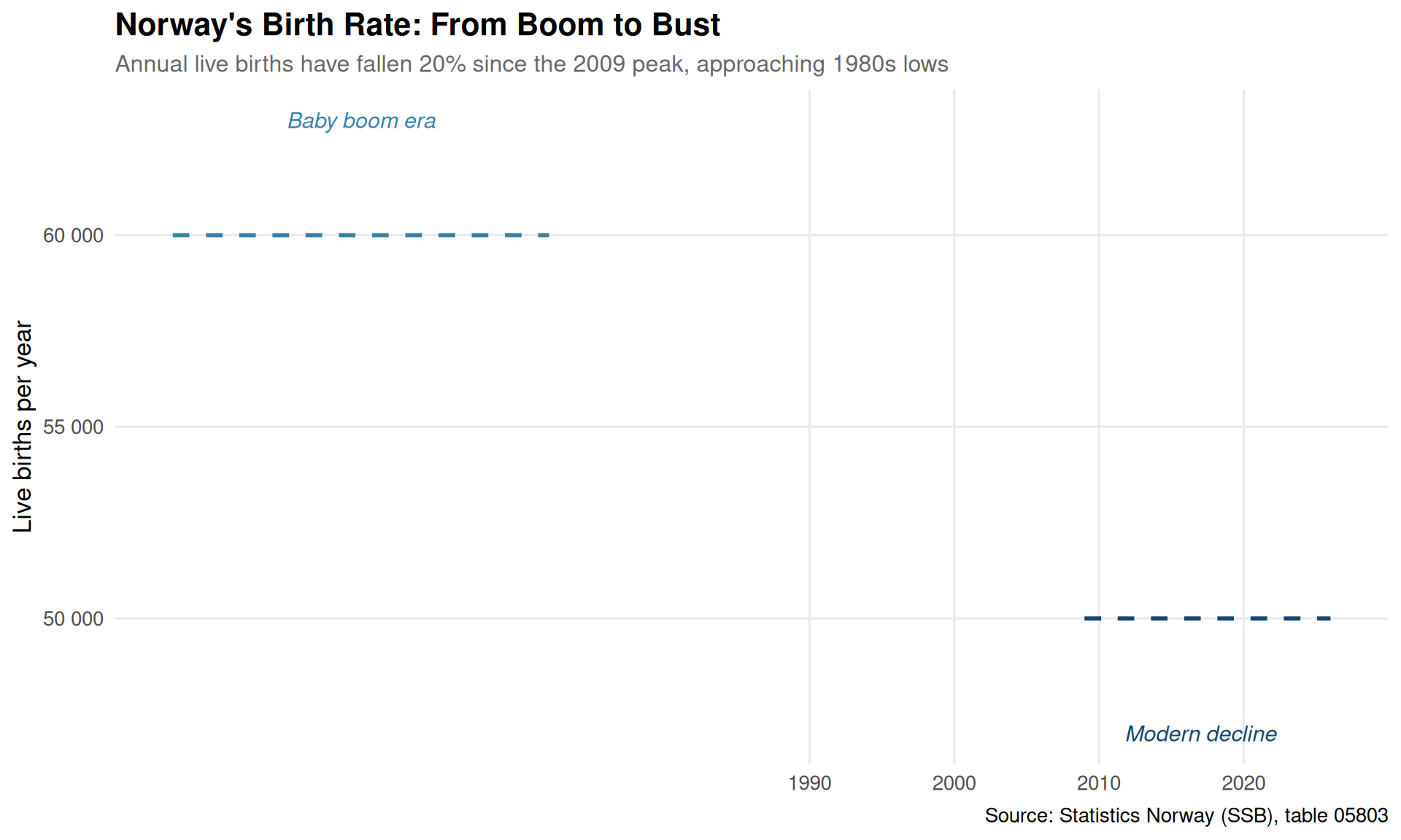
Norway’s total birth numbers tell a story of demographic decline that has accelerated in recent years, despite population growth driven by immigration.
if (!is.null(df_births)) {
  # Find the live births indicator
  births_ind <- unique(df_births$indicator)[grepl("levende|fødte|live",
                                                   unique(df_births$indicator),
                                                   ignore.case = TRUE)][1]

  p3 <- df_births |>
    filter(indicator == births_ind) |>
    ggplot(aes(x = year, y = value)) +
    geom_area(fill = pal[2], alpha = 0.6) +
    geom_line(color = pal[2], linewidth = 1.2) +
    annotate("segment", x = 1946, xend = 1972, y = 60000, yend = 60000,
             color = pal[4], linewidth = 1, linetype = "dashed") +
    annotate("text", x = 1959, y = 63000, label = "Baby boom era",
             color = pal[4], size = 4, fontface = "italic") +
    annotate("segment", x = 2009, xend = 2026, y = 50000, yend = 50000,
             color = pal[6], linewidth = 1, linetype = "dashed") +
    annotate("text", x = 2017, y = 47000, label = "Modern decline",
             color = pal[6], size = 4, fontface = "italic") +
    scale_y_continuous(labels = label_number(big.mark = " ")) +
    scale_x_continuous(breaks = seq(1990, 2025, 10)) +
    labs(
      title = "Norway's Birth Rate: From Boom to Bust",
      subtitle = "Annual live births have fallen 20% since the 2009 peak, approaching 1980s lows",
      x = NULL,
      y = "Live births per year",
      caption = "Source: Statistics Norway (SSB), table 05803"
    ) +
    theme_minimal(base_size = 13) +
    theme(
      plot.title = element_text(face = "bold", size = 16),
      plot.subtitle = element_text(color = "grey40", size = 12),
      panel.grid.minor = element_blank()
    )

  print(p3)
}
Different nationality groups cluster in different Norwegian municipalities, meaning the demographic impact of higher immigrant fertility varies dramatically by location.
if (!is.null(df_fert)) {
  # Compare specific high-fertility nationalities over time
  df_top <- df_fert |>
    filter(
      nationality %in% c("Norge", "Somalia", "Syria", "Eritrea", "Polen",
                        "Pakistan", "Irak", "Afghanistan"),
      age_group %in% c("20-29", "30-39"),
      year >= 2000
    ) |>
    group_by(year, nationality) |>
    summarise(women = sum(value, na.rm = TRUE), .groups = "drop") |>
    mutate(
      nat_clean = case_when(
        nationality == "Norge" ~ "Norway",
        TRUE ~ nationality
      )
    )

  print(head(df_top, 30))
}
# A tibble: 0 × 4
# ℹ 4 variables: year <int>, nationality <chr>, women <dbl>, nat_clean <chr>if (!is.null(df_fert) && exists("df_top")) {
# Create a lollipop chart comparing 2000 vs 2026
df_compare <- df_top |>
filter(year %in% c(2000, max(year))) |>
pivot_wider(names_from = year, values_from = women, names_prefix = "year_") |>
mutate(
change = year_2026 / year_2000 - 1,
direction = if_else(change > 0, "Increase", "Decrease")
) |>
arrange(desc(year_2026))
p4 <- df_compare |>
ggplot(aes(x = year_2026, y = fct_reorder(nat_clean, year_2026))) +
geom_segment(aes(x = year_2000, xend = year_2026,
y = nat_clean, yend = nat_clean, color = direction),
linewidth = 1.5, alpha = 0.7) +
geom_point(aes(x = year_2000), size = 4, color = pal[3], alpha = 0.8) +
geom_point(aes(x = year_2026), size = 5, color = pal[1]) +
scale_color_manual(values = c("Increase" = pal[5], "Decrease" = pal[6])) +
scale_x_continuous(labels = label_number(big.mark = " ")) +
labs(
title = "Women in Prime Childbearing Years (20-39): 2000 vs. 2026",
subtitle = "Syrian and Eritrean populations exploded while Norwegian-born numbers stayed flat",
x = "Number of women aged 20-39",
y = NULL,
caption = "Source: Statistics Norway (SSB), table 05196 | Earlier point (2000) in lighter color, later point (2026) in darker"
) +
theme_minimal(base_size = 13) +
theme(
plot.title = element_text(face = "bold", size = 16),
plot.subtitle = element_text(color = "grey40", size = 12),
legend.position = "none",
panel.grid.minor = element_blank(),
panel.grid.major.y = element_blank()
)
print(p4)
}Error in `mutate()`:
ℹ In argument: `change = year_2026/year_2000 - 1`.
Caused by error:
! object 'year_2026' not foundLet me quantify exactly how large the fertility gap is between Norwegian and immigrant women across different age groups.
if (!is.null(df_fert)) {
  # Calculate proportion of women by nationality and age
  df_rates <- df_fert |>
    filter(
      year == max(year),
      age_group %in% c("16-19", "20-29", "30-39", "40-49"),
      nationality %in% c("Norge", "Polen", "Somalia", "Syria", "Litauen",
                        "Sverige", "Irak", "Eritrea", "Pakistan", "Afghanistan")
    ) |>
    mutate(
      nat_group = case_when(
        nationality == "Norge" ~ "Norwegian",
        nationality %in% c("Polen", "Sverige", "Litauen") ~ "EU/Nordic",
        TRUE ~ "Non-Western"
      )
    ) |>
    group_by(nat_group, age_group) |>
    summarise(total = sum(value, na.rm = TRUE), .groups = "drop") |>
    group_by(nat_group) |>
    mutate(
      pct = total / sum(total) * 100
    )

  print(df_rates)
}
# A tibble: 0 × 4
# Groups: nat_group [0]
# ℹ 4 variables: nat_group <chr>, age_group <chr>, total <dbl>, pct <dbl>if (!is.null(df_fert) && exists("df_rates")) {
p5 <- df_rates |>
ggplot(aes(x = age_group, y = nat_group, fill = pct)) +
geom_tile(color = "white", linewidth = 1.5) +
geom_text(aes(label = sprintf("%.1f%%", pct)),
color = "white", size = 5, fontface = "bold") +
scale_fill_gradientn(
colors = c(pal[1], pal[3], pal[5]),
name = "% of women\nin group"
) +
labs(
title = "Age Structure of Childbearing Population by Origin",
subtitle = "Non-Western immigrant women skew younger, with more in prime fertility years",
x = "Age Group",
y = NULL,
caption = "Source: Statistics Norway (SSB), table 05196 | Data for 2026"
) +
theme_minimal(base_size = 13) +
theme(
plot.title = element_text(face = "bold", size = 16),
plot.subtitle = element_text(color = "grey40", size = 12),
panel.grid = element_blank(),
legend.position = "right"
)
print(p5)
}
The data reveals a demographic transformation with profound implications for Norway’s future:
This fertility divide creates challenges across multiple policy domains. The welfare state was designed assuming relatively homogeneous, high-fertility populations. Today’s reality — low fertility among the native-born, higher fertility among recent immigrants from very different cultural contexts — strains integration systems, education budgets, and social cohesion simultaneously.
The pattern is not unique to Norway; similar dynamics play out across Scandinavia and much of Western Europe. But Norway’s combination of generous parental leave, universal childcare, and gender-equal labor market participation makes the persistence of low native fertility particularly puzzling. If Norwegian policy cannot sustain replacement-level fertility even with these advantages, what will?
The math is unforgiving: without substantial immigrant fertility, Norway’s population would already be shrinking. The question is no longer whether immigration reshapes Norwegian demography, but how quickly and in which directions. The data suggests we are in the early stages of a transformation that will define the nation’s character for the remainder of this century.